A particular Gaussian mixture model for clustering and its ...

More documents

Recommendations

Info

H. SahbiConsider a chunk {µ ip }i=1 N and fix {µ jk, k ̸= p} N j=1 ,theobjective function (7) is linear in terms of {µ ip } and canbe solved, with respect to this chunk, using linear programming.Only one equality constraint ∑ i µ ip = 1 is takeninto account in the linear programming problem as the otherequality constraints in (6) are independent from the chunk{µ ip }.We can further reduce the size of the chunk {µ ip }i=1 N toonly two parameters. Given i 1 , i 2 ∈ {1,...,N}, we canrewrite (7) as:min 2 ( µ i1 p c i1 p + µ i2 p c i2 p)+ bµ i1 p, µ i2 ps.t µ i1 p + µ i2 p = 1 − ∑µ ipi ̸= i 1 ,i 20 ≤ µ i1 p ≤ 10 ≤ µ i2 p ≤ 1,here b is a constant independent from the chunk {µ i1 p,µ i2 p}(see 7). When c i1 p = c i2 p the above objective function andthe equality constraints are linearly dependent, so we have aninfinite set of optimal solutions; any one which satisfies theconstraints in (9) can be considered. Let us assume c i1 p ̸=c i2 p and denote d = 1 − ∑ i ̸= i 1 ,i 2µ ip , since µ i2 p = d −µ i1 p, the above linear programming problem can be writtenas:minµ i1 p (c i1 p − c i2 p)µ i1 ps.t max(d − 1, 0) ≤ µ i1 p ≤ min(d, 1)(9)(10)Depending on the sign of c i1 p − c i2 p, the solution of (10) issimply taken as one of the bounds of the inequality constraintin (10). At this stage, the parameters {µ 1p ,...,µ Np } whichsolve (7) are found by solving iteratively the trivial minimizationproblem (10) for different chunks, as shown inAlgorithm1,Algorithm1(p,µ)Do the following steps ITERMAX1 iterationsSelect randomly (i 1 , i 2 ) ∈{1,...,N} 2 .(c i1 p, c i2 p) ←− (8).if (c i1 p − c i2 p < 0) µ i1 p ←− min(d, 1) (see 10)else µ i1 p ←− max(d − 1, 0)µ i2 p ←− d − µ i1 p (see 9)endDoreturn (µ i1 p,...,µ iN p)and the whole QP (6) is solved by looping several timesthrough different cluster indices as shown in Algorithm2.For a convex form of the QP (6) and for a large value of ITER-MAX1 and ITERMAX2, each subproblem will be convexand the convergence of the decomposition algorithms (1,2) isguaranteed as also discussed for support vector machine training(Platt 1999). In practice ITERMAX1 and ITERMAX2are set to C and N 2 respectively.Algorithm2Set {µ} to random values.Do the following steps ITERMAX2 iterationsFix p in {1,...,C}, update µ 1p ,…,µ Np using:(µ 1p ,..., µ Np ) ←− Algorithm1(p,µ)endDo4.2 AgglomerationInitially, the algorithm described above considers an overestimatednumber of clusters (denoted C). This will resultinto several overlapping cluster GMMs which might be detectedusing a similarity measure for instance the KullbackLeibler divergence (Bishop 1995).Given two cluster GMMs p(x|y k ), p(x|y l ),forafixedɛ>0 we declare p(x|y k ), p(x|y l ) as similar if:∫X∥ p(x|yk ) − p(x|y l ) ∥ ∥ 2 dx < ɛ(11)As p(x|y k ) =〈ω k ,Φ σ (x)〉 and p(x|y l ) =〈ω l ,Φ σ (x)〉, wecan simply rewrite (11) as:∫X〈ω k − ω l ,Φ σ (x)〉 2 dx < ɛ(12)We can set the memberships in ω k , ω l such that ‖ω k ‖=‖ω l ‖=1. Now, from (12) it is clear that two overlappingGMMs correspond to two highly correlated hyperplanes inthe mapping space, i.e., 〈ω k ,ω l 〉 ≥ τ (for a fixed thresholdτ ∈[0, 1]).Regularization: notice that,∂〈 ω k ,ω l 〉∂σ≥ 0, (13)so the correlation is an increasing function of the scale σ .Assuming ‖w k ‖=‖w l ‖=1, it results that ∀ τ ∈[0, 1], ∃ σsuch that 〈ω k ,ω l 〉 ≥ τ.Let us define the following adjacency matrix:A k,l ={ 1 if〈ωk ,ω l 〉 ≥ τ0 otherwise(14)This matrix characterizes a graph where a node is a hyperplaneand an arc corresponds to two highly correlated hyperplanes(i.e., 〈ω k ,ω l 〉 ≥ τ). Now, the actual number of clusters isfound as the number of connected components in this graph.For a fixed threshold τ, the scale parameter σ acts as a regularizer.When σ is overestimated, the graph A ={A k,l } willbe connected resulting into only one big cluster whereas a123
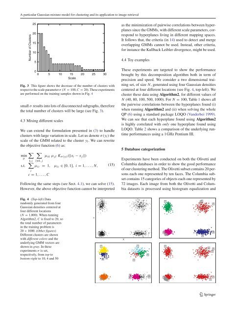
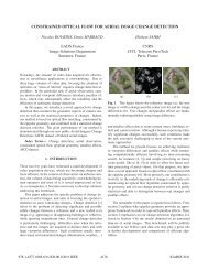
A particular Gaussian mixture model for clustering and its application to image retrievalNumber of Clusters25201510500 5 10 15 20 25 30ScaleFig. 3 This figure shows the decrease of the number of clusters withrespect to the scale parameter σ (N = 100, C = 20). These experimentsare performed on the training samples shown in Fig. 4small σ results into lots of disconnected subgraphs, thereforethe total number of clusters will be large (see Fig. 3).4.3 Mixing different scalesWe can extend the formulation presented in (3) to handleclusters with large variation in scale. Let us denote σ(y l ) thescale of the GMM related to the cluster y l . We can rewritethe objective function (6)as:minµs.t.∑k,i∑l̸=k, jµ ik µ jl K σ(yl )(‖x i − x j ‖)∑µ ic = 1, µ ic ∈[0, 1], i = 1,...,N,ic = 1,...,C(15)Following the same steps (see Sect. 4.1), we can solve (15).However, the above objective function cannot be interpretedas the minimization of pairwise correlations between hyperplanessince the GMMs, with different scale parameters, correspondto hyperplanes living in different mapping spaces.It follows that, the criteria (in 14) used to detect and mergeoverlapping GMMs cannot be used. Instead, other criteria,for instance the Kullback Leibler divergence, might be used.4.4 Toy examplesThese experiments are targeted to show the performancebrought by this decomposition algorithm both in term ofprecision and speed. We consider a two dimensional trainingset, of size N, generated using four Gaussian densitiescentered at four different locations (see Fig. 4, top-left). Wecluster these data using Algorithm2, for different values ofN (40, 80, 100, 500, 1000). For N = 100, Table 1 shows allthe pairwise correlations between the hyperplanes found (i)when running Algorithm2 and (ii) when solving the wholeQP (6) using a standard package LOQO (Vanderbei 1999).We can see that each hyperplane found using Algorithm2is highly correlated with only one hyperplane found usingLOQO. Table 2 shows a comparison of the underlying runtimeperformances using a 1 GHz Pentium III.5 Database categorizationExperiments have been conducted on both the Olivetti andColumbia databases in order to show the good performanceof our clustering method. The Olivetti subset contains 20 personseach one represented by ten faces. The Columbia subsetcontains 15 categories of objects each one represented by72 images. Each image from both the Olivetti and Columbiadatasets is processed using histogram equalization andFig. 4 (Top-left) Datarandomly generated from fourGaussian densities centered atfour different locations(N = 1,000). When runningAlgorithm2, C is fixed to 20, sothe total number of parametersin the training problem is20 × 1000. (Other figures)Different clusters are shownwith different colors and theunderlying GMM vectors areshown in gray. Intheseexperiments σ is set,respectively, from top tobottom-right to 10, 4 and 50YX123
Page 1 and 2: Soft ComputDOI 10.1007/s00500-007-0
Page 3: A particular Gaussian mixture model
Page 7 and 8: A particular Gaussian mixture model
Page 9 and 10: A particular Gaussian mixture model

A particular Gaussian mixture model for clustering and its ...

Create successful ePaper yourself

Delete template?

Save as template?