Analysis of genome-scale count data in Bioconductor

Analysis of genome-scalecount data in BioconductorMark D. Robinson 1,2 and Davis J. McCarthy 11Bioinformatics Division, The Walter and Eliza Hall Institute of Medical Research2Epigenetics Laboratory, Garvan Institute of Medical ResearchBioC 2010

Outline1. Applications2. Summarization3. Statistical models for count data4. “Normalization”5. Sharing information over entire dataset6. Statistical testing7. Other considerations – error model and morecomplex designs(Current) Bioconductor tools:baySeq, DEGseq, DESeq, edgeRPreliminaries(~40min)Practical(~20min)Moreadvancedtopics(~30min)Practical(~30min)

Sequencing experiments used for:Sequence of(mapped) reade.g. genome sequencing,SNP/mutation mapping,genomic rearrangements,etc.Position of mappedreade.g. RNA-seq, tag-seq forexpression, ChIP-seq forTF binding or histonemodifications, MeDIP-seqfor DNA methylation, etc.

Applications• Differential gene expression: RNA-seq,“Tag”-seq, etc.• Differential enrichment: histonemodifications, other types of “enrichment”-based sequencing e.g. ChIP-seq, MeDIPseq,etc.• Analyses of changes in other tables ofcounts: e.g. peptide counts from MS/MSexperiments, metagenomics experiments.

Example:RNA-seq(or similar)for geneexpression

Example:Enrichment of subsetof the genome (e.g.ChIP for histonemodifications or DNAmethylation)

Summarization

SummarizationCDS CDS CDS CDSFigure 2Coding Sequence Exons Introns Splice Juncons

What does genome-scale count• e.g. RNA-seqdata look like?Tag ID! A1! A2! A3! A4! B1! B2! B3!ENSG00000124208! 478! 619! 628! 744! 483! 716! 240!ENSG00000182463! 27! 20! 27! 26! 48! 55! 24!ENSG00000125835! 132! 200! 200! 228! 560! 408! 103!ENSG00000125834! 42! 60! 72! 86! 131! 99! 30!ENSG00000197818! 21! 29! 35! 31! 52! 44! 20!ENSG00000125831! 0! 0! 2! 0! 0! 0! 0!ENSG00000215443! 4! 4! 4! 0! 9! 7! 4!ENSG00000222008! 30! 23! 29! 19! 0! 0! 0!ENSG00000101444! 46! 63! 58! 71! 54! 53! 17!ENSG00000101333! 2256! 2793! 3456! 3362! 2702! 2976! 1320!…"… tens of thousands more tags …"

Statistical models for countdata

Count data• Count data (e.g. RNA-seq) is discrete, notcontinuous• Statistical methods designed formicroarrays are not directly applicable• Two options:Transform count dataand apply standardmethodologyAnalyze using modelsfor count data

Count data• BUT we have learned much from theanalysis of microarray data• Methods that share information over thewhole dataset generally:– stabilize parameter estimation– improve performance of making inferences

Poisson arises naturally frommultinomial samplingDNApopulation• Take sample• Sequence DNALibrary 1Gene 1 λ 1Gene 2 λ 2Gene 3 λ 3Gene 4 λ 4Gene 5 λ 5Gene 6 λ 6…

Reads for a single gene (singlelibrary) are binomial distributedLibrary 1…Gene i λ i…Y i ~ Binomial( M, λ i )Y i - observed number of reads for gene iM - total number of sequencesλ i - proportionLarge M, small λ i approximated well by Poisson( µ i = Mλ i )

Technical replicationDNApopulationLibrary 1 Library 2• Take anothersample fromsame pool• SequenceDNA

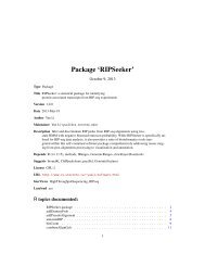
Robinson and Oshlack Genome Biology 2010, 11:R25http://genomebiology.com/2010/11/3/R25Poisson replication induces avuvuzela-shaped “MA”-plotRobinson and Oshlack Genome Biology 2http://genomebiology.com/2010/11/3/R2The trimmed mean of M-values normalization methodThe total RNA production, S k ,cannotbeestimateddirectly, since we do not know the expression levels andAnd the theorytrue lengths of every gene. The However, trimmed mean the relative of M-values RNAnThe validates total RNA that production, thisproduction of two samples, f k =S k /S k’ , essentially a globalfold change, can more easily be determined. we do not We know pro-thS kdirectly, behaviour sinceshouldtrue exist: lengths M ispose an empirical strategy that equatesof everythegene.overallHowproduction essentially of a two logrelative-riskfold change, can more easilysamples, f k =expression levels of genes between samples under thebalassumption that the majority of them are not DE. Onepose an empirical strategy thsimple yet robust way to estimateexpressionthelevelsratioofofgenesRNA productionuses a weightedassumption trimmed that mean theof majority the log ofPower (to detect betwexpression ratios (trimmedchanges)simple meanofMvalues(TMM)).is higher atyet robust way to estimatFor sequencing data, we definehigherduction thecountsuses gene-wise a weighted log-foldchangesas:trimImplications forexpression ratios (trimmed meaFor downstream sequencing data, we defineYgk N k changes as:M g / analysis.log 2Ygk / N k Ygk N kM g /log 2and absolute expression levels:Y gk / N k and absolute expression levels:Ag 1 log Ygk Nk YgkNk Yg22’ for 0Ag 1 log Ygk Nk YgkN22To robustly summarize the observed M values, wetrim both the M values and the A values before taking

Statistical models• For count data, variance increaseswith mean• Starting point: Poisson model• Poisson has simplest meanvariancerelationship

Poisson• Variance is equal to the mean• One-parameter model: mean for eachgene• M = library sizeY i ~ Pois( µ i )µ i = M * λ i• λ i = relative contribution of gene i

Poisson describes technicalvariance• Marioni et al (2008) show that there islittle technical variance in RNA-seq• Poisson model is (probably) adequatefor assessing DE when there are onlytechnical reps• But this is not the end of the story …

Biological replication2 or more independent DNA populations fromthe same experimental conditionGenerally, experimenters will want biologicalreplication for generalizable results

Overdispersion: extra-Poissonvariation• If there are ANY further sources ofvariation, there is more variation indata than Poisson model can accountfor• Poisson model underestimatesvariation -> false positives• Need a model that can account forthis extra variation

Overdispersion is present in real dataMean-variance plot for slime-mould dataset hr00 and hr24 (2 vs 2)Genevariance(pooled)(log10scale)Gene mean expression level (log10 scale)Comparing expression levels from Dictyostelium discoideum at hr00 and hr24 – two biological replicates at each time point.RNA-seq data from Parikh et al. Genome Biology 2010, 11:R35 http://genomebiology.com/2010/11/3/R35

Sources of variation: technical andbiological• Technical: same pool of RNA sequencedseparately (e.g. different lanes)• Biological: RNA from different biologicalsources (e.g. individuals) under the sameexperimental conditions• Other: extra-Poisson variation alsointroduced by other processes, e.g.different library preparations, protocols etc.

Natural extension to Poisson:negative binomial model• Introduce the dispersion parameterY i ~ NB( µ i , ϕ i )• Still have mean expression levelµ i = M * λ i• M = library size, λ i = “conc” of gene DNA• Variance is a quadratic function of mean:Var( Y i ) = µ i ( 1 + µ i ϕ i )

Coefficient of variation• Dispersion is squared coefficient ofvariation• Measure of similarity/variability btwsamples• E.g. dispersion = 0.2 -> coef of var = 0.45• Interpretation: true expression levels ofgenes vary by 45% btw replicates• Separate biological and technical variation

Problem: small sample size• RNA-seq experiments will typically havesmall sample sizes (e.g. n=7)• Standard methods for estimating thedispersion for each gene produce veryunreliable estimates• Lesson from microarrays: shareinformation between genes (variancestructure) to improve inference

Common dispersion model• One approach: use same value forthe dispersion for all genes• Estimate using all genes in dataset(conditional max likelihood)• Produces a reliable estimate• Nice biological interpretation, but canbe heavy handed

Normalization

High read number is relevant for RNA-Seq because our ability toreliably detect and measure rare, yet physiologically relevant, RNAspecies (those with abundances of 1–10 RNAs per cell) depends onthe number of independent pieces of evidence (sequence reads)obtained for transcripts from each gene. This constraint influencedour sequencing strategy, choice of instrument and choice of the25-bp read length.The sensitivity of RNA-Seq will be a function of both molar concentrationMortazaviand transcriptetlength.al. 2008We thereforeNaturequantifiedMethodstranscriptlevels in reads per kilobase of exon model per million mapped reads(RPKM) (Fig. 1a,c). The RPKM measure of read density reflectsthe molar concentration of a transcript in the starting sample bynormalizing for RNA length and for the total read number in themeasurement. This facilitates transparent comparison of transcriptlevels both within and between samples.Wang et al. 2008 Nature Reviews GeneticsBut, this is not the full story. Examination of a well-characterized locusData from a 21-million-read transcriptome measurement of adultmouse skeletal muscle (Fig. 1b,c) illustrate some key characteristicsof our results. Myf6 (also known as Mrf4) is a much-studied29and plong (transc(~0.5transca dyntion. Sand qsequedetecbase (valueimpacthe coRPKMin conlute trthe baand thabout

Kidney and Liver RNA have verydifferent compositionlog 2 (Kidney1 N K1 ) ! log 2 (Kidney2 N K2 )Density−6 −4 −2 0 2 4 60.0 0.4 0.8Alog 2 (Liver N L ) ! log 2 (Kidney N K )Density−6 −4 −2 0 2 4 60.0 0.2 0.4B!!!!!!!!!!!!!!!!!!!!!!!!!!!!!!!!! !!!!!!!!!!!!!! !!!!!!!!!!!!!!!!!!!!!!!!!!!!!!!!!!!!!!!!!!!!!!!!!!!!!!!!!!!!!!!!!!!!!! !!!!!!!!!!!!!!!!!!!!!!!!!!!!!!!!!!!!!!!!!!!!!! !!! !!!!!!!!!!!!!!!!!!!!!!!!!!!!!!!!!!!!!!!!! !!!!!!!!!!!!!!!!!!!!!!!!!!!!!!!!!!!!!!!! !!!!!!!!!!!!!!!!!!!! !!!!!!!!!!!!!!!!!!!!!!!!!!!!!!!!!!!!!!!!!!!!!!!! !!!!!!!!!!!!!!!! !!!!!!!!!!!!!!!!!!!!!!!!!!!!!!!!!!! !!!!!!!!!!!!!!!!!!!!!!!!!!!!!!!!!!!!!!!!!!!!!!!!!!!!!!!!!!!!!!!!!!!!!!!!!!!!!!!!!!!!!! !!!!!!!!!!!!!!!!!!!!!!!!!!!!!!!!!!!!!!!!!!!!!!!!!! !!!!!!!!!!! !!!!!!!!!! !!!!!!!!!!!! !!!!!!!!!!!!!!! ! !!!!!!!!!!!!!!! !!!!!!!!!!!!!!!!!!!!!! !!!!! !!!!!!!!!!!!!!!!!!!!!!!!!!!!!!!!!!!!!!!! !!!!!!!!!!!!!!!!!!!!!!!!!!!!!!!!!!!!!!!!!!!!!!!!!!!!!!!!!!!!!!!!!!!!!! !!!!!!!!!!!!!!!!! !!!!!!!!!!!!!!!! !!!!!!!!!!!!!!!!!!!!!!!!!!!!!!!!!!!!!!!!!!!!!!!!!!!!!!!!!!!!!!!!!!!!!!!!!!!!!!!!! !!!!!!!!!!!!!!!!!!!!!!!!!!!!!!!!!!!!!! !!!!!!!!!!!!!!!!!!!!!!!!!!!!!!!!!!!!!!!!!!!!!!!!! !!!! !!!!!!!!!!!!!!!!!!!!!!!!!!!!!!!!!!!!!!!!!!!!!!!!!!!!!!!!!!!!!!! !!!!!!! !!!!!!!! !!!!!!!!!!!!!!!!!!!!!!!!!!!!!!!!!!!!!!!!!!!!!!!!!!!!!!!!!!!!!!!!!!!!!!!!!!!!!!!!!!!!!!! !!!!!!!!!!!!!!!!!!!!!!! !!!!!!! !!!!!!!!!!!!! !!!!!!!!!!!! !!!!!!!!!!!!!!!!!!!!!!!!!!!!!!!!!!!!!!!!!!!!!!!!!!!!!!!!!!!!!!!!!!!!!!!!!!!!!!!!!!!!!!!!!!!!!!!!!!!!!!!!!!!!!!! !! !!!!!!!!!!!!!!!!!!!!!!!!!!!!!!!!!!!!!!!!!!!!!!!!!!!!!!!!! !!!!!!!!!!!!!!!!!!!!!!!!!!!!!! !!!!!!!!!!!!!!!!!! !!!!!!!!!!!!!!!!!!! !!!!!!!!!!!!!!!!!!!!!!!!!!! !!!!!!!!!!!!!!!!!!!!!!!!!!!!!!!!!!!!!!!!!!!!!!!!!!!!!!!!!!!!!!!!!!!!!!!!!!!!!!! !!!!!!!!!!!!!!!!!!!!! !!!!!!!!!!!!!!!!!!!!!!!!!!!!!!!! !! !!!!!!!!!!!!!! !!!!!!!!!!!!!!!!!!!!!!!!!!!!!!!!!!!!!!!!!!!!!!!!!!!!!!!!! !!!!!!!!!!!!!!!!!!!!!!!!!!!!!!!!!!!!! !!!!!!!!!!!!!!!!!!!!!!!!!!!!!!!!!!!!! !!!!!!!!!!!!!!!!!! !!!!!! !!!!!!!!!!!!!!!!!!!!!!!!!!!! !!!!!!!!!!!!!!! !!!!!!!!!!!!! !!!!!!!!!!!!!!!!!!!!!!!!!!!!!!!!!!!!!!! !!!!!!!!!!! !!!!!!!!!!!!!!!!! !!!!!!!!!!!!!!!!!!!!!!! !!!!!!!!!!!!!!!!!!!!!!!!!!!!!!!!!!!!!!!!!!!!!!!!!!!!!!!!!!!!!!!!!!!!!!!!!!!!!!!!!!!!!!!!! !!!!!!!!!!!!!!!!!!!!!!!!!!!!!!!!!! !!!!!!!!!! !!!!!!!!!!!!!!!!!!!! !!!!!!!!!!!!!!! !!!!!!!!! !!!!!!!!!!!!!!!!!!!!!!!!!!!!!!!!!!!!!!!!!!!!!!!!!!!!!!!!!!!!!!!!!!!!!!!!!!!!!!!!! ! !!!!!!! !!!!!!!!!!!! !!!! ! !!!!!!!!!!!!!!!!!!!! !!!!!!!!!!!!!!!!!!!!!!!!!!!!! !!!!!! !!!!!!!!!!!!!!!!!!!!!!!!!!!!!!!!!!!!!!!!!!!!!!!!!!! !!!!!!!!!!!!!!!!!!!!!!!!!!!!!!!!!!!!!!! !! !!!!!!!!! !!!!!!!!!!!!!!!!!!!!!!!!!!!!!!!!!!!!!!!!!!!!!!!!!!!!!!!!!!!!!!! !!!!!!!!! !!!!!!!!!!!!!!!!!!! !!!!!!!!!!!!!!!!!!!!!!!!!!!!!!!!!!!!!!!!!!!!!!!!!!!!!!!!!!!!!!!!!!!!!!!!!!!!!!!!!!!! !!!!!!!!!!!!!!!!!! !!!!!!!!!!!!!!!!!!!!!!! !!!!!!!!!!!!!!!!!!!!!!!!!!!!!!!!!!!!!!!!!!!!!!! !!!!!!!!!!!!!!!!!!!!!!!!!!!!!!!!!!!!!!! !!!!!!!!! !!!!!!!!!!!!!!!!!!!!!!!!!!!!!!!!!!!!!!!!!!!!!!!!!!!! !!!!!!!!!!!!!!!!!!!! !!!!!!!!!!!!!!!!!!!!!!!! !!!!!!!!!!!!!!!!!!!!!!!!!!!!!!!!!!!!!!!!!!!!!!!! !!!!!!!!!!!!!!!!!!!!!!!!!!!!!!!!!!!!!!!!!!!!!!!!!!!!!!!!!!!!!!!!!!!!!!!!!!!! !!!!!!!!!!!!!!! !!!!!!!!!!!!!!!!!!!!!!!!!! !!!!!!!!!!!!!!!!!!! !! ! !!!!!!!!! ! !!! !!!! !!!!!!!!!!!!!!!!!!!!!!! !!!!!!!!!!!!!!! !!!!!!!!!!!!!!!!!!!!!!!!!!!!!!!!!!!!!!!! !!!!!!!!!!!! !!!!!!!!!!!!!!!!!!!!!!! !!!!!!!! !!!!!!!!!!! !!!! !!!!!!!!!! ! !!!!!!!!!!!!!!!!!!!!!!!!!!!!!!!!!!!!!!!!!!!!!!!!!!!!!!!!!!!!!!!!!!!!!!!!!!!!!!!!!! !! !!! !!!!!! !!!!!! !!!!!!!! !!!!!!!!!!!!!!!!!!!!!!!!!!!!!!!!!!!! !!!!!! !!!!!!!!!!!!!!!!! !!!!!!!!!!!!!!! !!!!!!!!!!!!!!!!!!!!!!!!!!!!!!!!!!!!!!!!!!!!! !!!!!!!!!!!!!!!!!!!!!!!!! !!!!!!!!!!!!!!!!! ! !!!!!!!!!!!!!!!!!! !!!!!! ! !!!!!!!!!!!!!!!!!!!!! !!!!!!!!!!!!!!! !!!!!!!!!!!!!!!!!!!!!!!!! ! !!!!!!!!!!!!!!!!!!!!!!!!!!!!!!!!!!!!!!!!!!!!!!!!!!!!!!!!!!!!!!!!!!! !!!!!!!!!!!!!!!!!!!!!!!!!!!!!!!!!!!!!!!!!!!!!!!!!!!!!!!!!!!!! !!!!!!!!!!!!!!!!!!!!!!!!!!!!!!!!!!! !!!!!!!!!!!!!!!!!!! !!!!!!!!!!!!!!!!!!!!!!!!!! !!!!!!!!!!!!!!!!!!!!!!!!!!!!!!!!!!!!!!!!!!!!!!!!!!!! ! !!!!!!!!!!!!!!!!!!!!!!!!!!!!!!!!!!!!!!!!!!!!!!!!!!!!!!!!!!!!!! !!!!!!!!!!!!!!!!!!!!!!!!!!!!!!!!!!!!!!!!!!!!!!!!!!!!!!!!!!!!!!!!!!!!!!!!!!!!!!!!!!!!!!!!!!!!!!!!!!!!!!!!!!!!!!!!!!!!!!!!!!!!!!!!!!!!!!!!!!!!!!!! !! !!!!!!!!!!!!!!!!!!! !!!!!!!!! ! !!!! !!!!! !!!!!!!!!!!!! !!!!!!!!!!!!!!!!!!!! !!!!!!!!!!!!!!!!!!!!!!!!!!!!! !!!!!!!!!!!!!!!!!!!!!!!!!!!!!!!!!!!!!!! !!!!!!!!!!!!!!!!!!!!!!!!!!!!!!!!!! !!!!!!!!!!!!!!!!!!!!!!!!!!!!!!!!!!!!!!!!!!!!!!!!!!! !!!!!!!!!!! !!!!! !!!!!!!! !!!!!!!!!!!!!!!!!!!!!!!!!!!!!!!!!!!! !!!!!!!!!!!!!!!!!!!!!!!!!!!!!!!!! !!!!!!!!! ! !!!!!!!!!!!!!!!!!!!!!!!!!!!!!!!!! !!!!!!!!!!!!!!!!!!!!!!!!!!!!!!!!!!!!!!!!!!!!!!!!! !!!!!!!!!!!!!!!!!!!!!!!!!!!!!!!!!!!!!!!!!!!!!!! !!!!!!!!!!!!!!!!!!!!!!!!!!!!!!!!!!!!!!!!!!!!!!!!!!!!!!!!!!!!!!!!!!!!!!!!!!!!!!!!!! !!!!!!!!!!!!!!!!!!!! !!!!!!!!!!!!!!!!!!!!!!!!!!!!!!!!!!!!!!!!!!!!!!!!!!!!!!!!!!!!!!!!!!!!!!!!!!!!!!! !!!!!!!!!!!!!!!!!!!!!!!!!!!!!!!!!!!!!!!!!!!!!!!!!!!!!!!!!!!!!!!!!!!!!!!!!!!!!! !!!!!!!!!!!!!!!!!!!!!!!!!!!!!!!!!!!!!!!!!!!!!!!!!!!!!!!!!!! !!!!!!!! !!!!!!! !!!!!!!!!!!!!!!!!!!!!!!!!!!!!! !!!!! !!!!!!!!!!!!!!!!!!! ! !!!!!!!!!!!!!!!!!!!!!!!!!!!!!!!!!!!!!!! !!!!!!!!!!!!!!!!!!!!!!!!!!!!!!!!!!!!!!!!!!!!!!!!!!!!!!!!!!!!!!!!!!!!!!!!!!!!!!!!!!!! !!!!!!!!!!!!!!!!!!!!!!!!!!!!!!!!!!!!!!!!!!!!!!! !!!!!!!!!!!!!!!!!!!!!!!!!!!! !!!!!!!!!! !!!!!!!!!!!!!!!!!!!!!!!!!!!!!!!!!!!!!!!!!!!!!!!!!!!!!!!!!!!!!!!!!!!!!!!!!!!!!!!!!!!!!!!!!!!!!!!!! !!!!!!!!!!!!!!!!!!!!!!!!!!!!!!!!!!!!! !!!!!!!!!!!!!!!!!!!!!!!!!!!!!!!!!!!!!!!!!!!!!!!!!!!!!!!!!!!!!!!!!!!!!!!!!!!!!!!!!!!!!!!!!! !!!!!!!!!!!! !!!!!!!!!!!!!!!!!!!!!!!!!!!!!!!!!!!!!!!!!!!!!!!!!!!!!!!!!!!!!!!!!!!!!!!!!!!!!!!!!!!!!!!!!!!!!!!!!!!!!!!!!!!!!!!!!!!!!!! !!!!!!!! !!!!!!!!!!!!!!!!!!!!!!!!! !!!!!!!!!!!!!!!!!!!!!!!!! !!!!!!!!!!!!!!!!!!!!!!!!!!! !!!!!!!!!!!!!!!!!!!!!!!!!!! !!!!!!!!!!!!!!!!!!!!!!!!!!!!!!!!!!!!!!!!!!!!!!!!!!!!!!!!!!!!!!!!!!!!!!!!!!!!!!!!!! ! !!!!!!!!!!!!!!!!!!!!!! !!!!!!! !!!!!!! !!!!!!!!!! !! !!!!!!!!!!!!!!!!!!!!!!!!!!!!!!!!!! !!!!!!!!!!!!!!!!!!!!!!!!!! !!!!!!!!!!!!!!!!!! !!!!!!!!!!!!!!!!!!!!!!!!!!!! !!!!!!!!!!!!!!!!!!!!! !!!!!!!!!!!!!!!!!!!!!!!!!!!!!!!!!!!!!!!!!!!!!!!!!!!!!!!!!!!!!!!!!!!!!!!!!!!!!!!!!!!!!!!!!!!!!!!!!!!!!!!!!!!!!!!!!!!!!!!!!!!!!!!!!!!!!!!!!!! !!!!!!!!!!!!!!!!!!!!!!!!!!!!!!!!!!!!!!! !!!!!!!!!!!!!!!!!!!!!!!!!!!!!!!! !!!!!!!!!!!!!!!!!!!!!!!!!!!!!!!!!!! !!!!!!!!!!!!!!!!!!!!!!!!!!!!!! !!!!!!!!!!!!!!!!!!!!!!!!!!!!!!!!!!!!!!!!! !!!! !!!!!!!!!!!!!!!!!!!!!!!!!!!!!!!!!!!!!!!!!!!!!!!!!!!!!!!!!!!!!!!!!!!!!!!!! !!!!!!! !!!!!!!!!!!!!!!!!!!!!!!!!!!!!!!!!!!!!!!!!!! !!!!!!!!!!!!!!!!!!!!!!! !!!!!!!!!!!!!!!! !!!!!!!!!!!!!!!!!!!!!!!!!! !! !!!!!!!!!!!!!!!!!!!!!!!!!!!!!!!!!!!!!!!!!!!!!!!! !!!!!!!!! !!!!!!!!!!!!!!!!!!!!!! !!!!!!!!!!!! ! !!!!!!!!!!!!!!!!!!!!!!!!!!!!!!!!!!!!!!!!!!!!!!!!!!!!!!!!!!!!!!!!!! !!!!!!!!!!! ! !!!!!!!!!!!!!!!!!!! !!!!!!!!!!!!!!!!!!!!!!!!!!!!!!!!!!!!!!! !!!! !!!!!!!!!!!!!!!!!!!!!!!!!!! !!!!! !! !!!!!!!!!!!!!!!!!!!!!!!!!!!!!!!!!!!!!!!!!!!!!!!!!!!!!!!!!!!!!!!!!!!!!!!!!!!!!!!!!!!!!!!!!!!!!!!!!!!!!!!!!! !! !!!!!!!!!!!!!!!!!!!!!!!!!!!!!!!!!!!!!!!!!!!!!!!! ! !!!!!!!!!!!!!!!!!!!!!!!!!!!!!!!!! !!!!!!!!!!!!!!!!!!!!!!!!!!!!!!! !!!!!!!!!!!!!!!!!!! !!!!!!!!!!!!!!!!!!!!!!! !!!! ! !!!!!!!!!!!!!!!!!!!!!! !!!!!!!!!!!!!!!!!!!!!!!!!!!! !!!!!!!!!!!!!!!!!!!!!!!!! !!!!!!!!!!!!!!!!!!!!!!!!!!!!!!!!!!!!!!!!!!!!!!!!!!!!!!!!!!!!!!!!!! !!!!!!!!!!!!!!!!!!!!!!!!!!!!!!!!!!!!!!!!!!!!!!!!!!!!!!!!!!!!!!!!!!!!!!!!!!!!!!!!!!!!!!!!!!!!!!!!!! !!!!!!!!!!!!!!!!!!!! !!!!!!!!!!!!!!!!!!!!!!!!!!!!!!!!!!!!!!!!!!!!!!!!!!!!!!!!!!!!!!!!!!!!!!!!!!!!!!!!!!!!!!!!!! !!!! !!!! !!!!!!!!!!!! !!!!!!!!!!!!! !!!!!! !!!!!!!!!!!!!!!!!!!!!!!!!!!!!!!!!!!!!!! !!!!!!!!!! !!!!!! !!!!!!!!!!!!!!!!!!!!!! !!!! !!!!!!!!!!!!!!!!!!!!!!!!!!!! !!!!!!!!!!!!!!!!!!!!!!!!!!!! !! !!!!! !!!!!!!!!!!!!!!!! !!!!!!!!!!!!!!!! !!!!!!!!!!!!!!!! !!!!!!!!!!!!!!!!!!!!!!!!!!!!!!!!!!!!!!!!!!!!!!!!!!!!!!!!!!!!!!!!!!!!!!!!!!!!!!!!!!!!!!!!!!!!!!!!!!!!!!!!!!!!!!!!!!!!!!!!!!!!!!!!!!!!!!!!!!!!!!! !!!!!!!!!!!!!!!!!!!!!!!!!!!!! !!!!!!!!!!!!!!!!!!!!!!!!!!!! !!!!!! !!!!!!!!!!!!!!!!!!!!!!!!!!!!!!!!!!!!!!!!!!!!!!!!!!!!!!!!!!!! !!!!!!!!!!!!!!!!!!!!!!!!!!!!!!!!!!!!!!!!!!!!!!!!!!!!!!!!!!!!!!! !!!!!!!!!!!! !!! ! !!!!!!!!!!!!!!!!!!!!!!!!!!!!! !!!!!!!!!!!!!!!!!!!!!!!!!!!!!!!!!!!!!!!!!!! !!!!!!!! !!!!!!!!!!!!!!!!!!!!!!!!!!!!!!!!!!!!!!!!!!!! !!!!!!!!!!!!!!!!!!!!!!!!!!!!!!!!!!!!!!!!!!!!!!! !!!!!!!!!!!!!!!!!!!!!!!!!!!!!!!!!!!!!!!!!!!!!!!!!!!!!!!!!!!!!!!!!!!!!!!!!!!!! !!!!!!!!!!!!!!!!!!! !!!!!!!! !!!!!!! !!!!!!!!!!!!!!!!!!!!!!!!!!!!!!!!!!!!!!!!!!!!! !!!!!!!!!!!!!!!!!!!!!!!!!!!!!!!!!!!!!!!!!!!!!!! !!!!!!!!!!!!!!!!!!!!!!!!!!!!!!!!!!!!!!!!!!!!!!!!!!!!!!!!!!!!!!!!!!!!!!!!!!!!!!!!!!!!!!!!!!!!!!!!!!!!!!!!!!!!!!!!!!!!!!!!!!!!!!!!!!!!!!!!!!!!!!!!!!!!!!!!!!!!!!!!!!!!!!!!!!!!!!!!!!!!!!!!!!!!!!!!!!!!!!!!!!!!!!!!!!!!!!!!!!!!!!!!!!!!!!!!!!!!!!!!!!!! !!!!!!!!!!!!!!!!!!!!!!!!!!!!!!!!!!!!!!!!!!!!!!!! !!!!!!!!!!!!!!!!!!! !!!!!!!!!!!!!!!!!!!!!!!!!!!!!!!!!!! !!!!! !!!!!! !!!!!!!!!!!!!!!!!!!!!!!!!!!!!!!!!!!!!!!!!!!!!! !!!!!!!!!!!!!!!!!!!! !!!!!!!!!!!!!!!!!!!!!!!!!!! !!!!!!!!!!!!! !!! !!!!!!!!!!!!!! !!!!!!!!!!!!!!!!!! !!!! !!!!!!!!!!!!!!!!!!!!!!!!!!!!!!! !!!!!!!!!!!!!!!!!!!!!!!!!!!!!!!!!!!!!!!!!!!! !!!!!!!!!!!!!!!!!!!!!!!!!!!!!!!!!!!!!!!!!!!!!!!!!!!!!!!!!! !!!!!!!!!!!!!!! !!!!!!!!!!! !!!! !!!!!!!!!!!!!!!!!!!!!!!!!!!!!!!!! !!!!!!!!! !!!!!!!!!!!!!!!!!!!!!!!!!!!!!! !!!!!!!!!!!!!!!!!!!!!!!!!!!!!!!!!!!!!!!!!!!!!!!!!!!!!!!!!!!! !!!!!! !!!!!!!!!!! !!!!!!!!!!!!!!!!!!!!!!!!!!!!!!!!!!!!!!!!!!!!!!!!!!!!!!!!!!! !!!!!!!!!!!! !!!!!!!!!!!!!!!!!!!!!!!!!!! !!!!! !!!!!!!!!!!!!!!!!!!!!!!!!!!!!!!!!!!!!!!!!!!!! !!!!!!!!!!!!!!!!!!!!!!! !!!!!!!!!!!!!!!!!!!!! !!!!!!!!!!!!!!! !!!!!!!!!!!!!!!!!!!!!!!!!!!!!!! ! !!!!!!!!!!!!!!!! !!!!!!!!!!!!! ! !!!!!!!!!!!!!!!!!!!!!!!!!!!!!!!!!!!!!!!!!!!!!!!! !!!!!!!!!! !!!!!!!!!!!!!!!!!!!!!!!!!! !!!!!!!!!!!!!!!!!!!!!!!!!!!! !!!!!!!!!! !!!!!!!!!!!!!!!!!!!!!!!!!!!!!!!!!!!!!!!!!!!!!!!! ! !!!!!!!!!!!!!!!!!!!!!!!!!!!!!!!!!!!!!!! !!!!!!!!!!!!!!!!!!!!!!!!!!!!!!!!!!!!!!!!!!!!!!!!!!!!!!!!!!!!!!!!!!!!!!!!!!!!!!!!!!!!!!!!!!!!!!!!!!!!!!!!!!!!!!!!!!!!!!!!!!!!!!!!!!!!!!!!!!!!!!!! !!!!!!!!!!!!!!!!!!!!!!!! !!!!!!!!!!!!!!!!!!!!!!!!! !!!!!!!!!!!!!!!!!!! !!!!!!!!!!!!!!!!!!! !!!!!!!!!!!!!! !!!!!!!!!!!! !!!!!!!!!!!!!!!!!!!!!!!!!!!!!!!!! !!!!!!!!!!!!!!!!!!!!!!!!!!!! !!!!!!!!!!!!!!!!!!!!!!!!!!!!!!! !!!!!!!!!!!!!!!!!!!!!!!!!!!!!!!!!!!!!!!!!!!!!!!!!!!!!!!!!! !!!!!!! !!!!!! !!!!!! !!!!!!!!!!!!!!!!!!!!!!!!!!!!! !!!!!!!!!!!!!!!!!!!!!!!!!!!!!!!!!!!!!!!!!!!!!!!!!!!!!!!!!!!!!!!!!!!!!!!!!!!!!!!!!!!!!!!!!!!!!!!!!!!!!!!!!!!!!!!!!!!!!!!!!!!!!!!!!!!!!!!!!!!!!!!!!!!!!!!!!!!!!!!!!!!!!!!!!!!!!!!!!!!!!!!!!!!!!!!!!!!!!!!!!!!!!!!!!!!!!!!!!!!!!!!!!!!!!!!!!!!!!!!!!!! !!!!!!!!!!!!!!!!!!!!!!!!! !!!!!!!!!!!!!!!!!!!!!! !!!!!!!!!!!!!!!!!!!!!!!!! !! !!!!!! !!!!!!!!!!!!!!!!!!!!!!!!!!!!!!!!!!!!!!!!!!!!! !!! !!!!!!!!!!!! !!!!!!!!! !!!!!!!!!!! !!!!!!!!!!!!!!!!!!!!!!!!!!!!!!!!!!!!!!!!!!!!! !!!!!!!! !!!!! !! ! !! !!!!!!!!!!!! !!!!!!!!!!!!!!!!!!!!!!!!!!!!!!!!!!!!!!!!!!!!!!!!!!!!!! !!!! !! !!!!! !!!!!!!!!!!!!!!!!!!!!!!!!!!!!!!!!!!!!!!!!!!!!!!!!!!!!!!!!!!!!!!!!!!!!!!!!!!!!!!!!!!!! !!!!!!!!!!!!!!!!!!!!!!!!!!!!!!!!!!!!!!!!!!! !!!!!!!!!!!!!!!!!!!!!!!!!!!!!!!!!!!!!!!!!!! !!!!!!!!!!!!!!!!!!!!!!!!!!!!!! ! !!!!!!!!!!!!!!!!!!!!!!!!!!!!!!!!!!!!!!!!!!!!!!!!!!!!! !!!!!!!!!!!!!!!! !!!!!!!!!!!!!!!!!!!!!!!!!!!!!!!!!!!!!!!!!!!!!!!!!!!!!!!!!!!!!!!!!!!!!!!!!!!!!!!!!!!!!!! !!!!!!!! !!!!!!!!!!!!!!!!!!!!!!!!!!!!!!!!! !!!!!!!!!!!!! !!!!!!!!!!!!!!!!!!!!!!!!!!!!!!!!!!!!!!!!!!!!!!!!!!!!!!!!!!!!!!!!!!!! !!!!!!!!!!!!!!!!!!!!!!!!!!!!!!!!!!!!!!!!!!!!!!!!!!!! ! !!!!!!!! !!!!!!!!!!!!!! !!!! !!!!! !!!!!!!!!!!!!!!!!!!! !!!!!!!!!!!!!!!!!!!!!!!!!!!!!!!!!!!!!!!!!!!!!!!!!!!! !!!!!!!!!!!!!!!!!!!!!!!!!!!!!!!!!!! !!!!!!!!!! !!! !!!!!!!!!!!!!!!!!!!!!!!!!! !!!!!!!!! !!!!!!!!!!!!!!!!!!!!!! !!!!!!!!!!!!!!!!! !!!!!!!!!!!!!!!!!!!!!!!!!!!!!!!!!!!!!!!! !!!!!!!!!! !!!!!!!!!!!!!!!!!!!!!! !!!!!!!!!!!!!!!!!! !!!!!!!!!! !!!!!!!!!!!!!!!!! !!!!!!!!!!!!!!!!!!!!!!!!!!!!!!!!!!!!!! !!!!!!!!!!!! !!!!!!!!!! !!!! !!!!!!! !!!!!!!!!!!!!!!!!!!!!!!!!!!!!!!!!!!!!!!!!!!!!!!!!!!!!!! !!!!!!!!!!!!!!! !!!!!! !!!!!!!!!!!!!!!!!!!!!!!!!!!!!!!!!!!!!!!!!!!!!!!!!!!!!!!!!!!!!!!!!!!!!!!!!!!!!!!!!!!!!!! !!!!!!!!!!!!!!!!!!!!!!!!!!!!!!!!!!!!!!!!!!!!!!!!!!!!!!!!!!!!!!!!!!!!!!!!!!!!!!!!!!!!!! !!!!!!!!!! ! !!!!!!!!!!!!!!! !!!!!!!!!!!!!!!!!!!!!!!!!!!!!!!!!!!!!!!!! !!!!!!!!!!!!!!!!!!!!!!!!!!!!!!!!!!!!!!!!!!!!!!!!!!!!!!!!!!!!!!!!!!!!!!!!!!!!!!!!!!!!!!!!!!!!!!!!!!!!!!!!!!!!!!!!!!!!!!!!!!!!!!!!!!!!!!!!!! !!!!!!!!!!!!!!!!!! !!!!!!!!!!!!!!!!!!!!!!!!! !!!!!!!!!!!!!!!!!!!!!! !!!!!!!!!!!!!!!!!!!!!!!!!!!!!!!!!!!!!!!!!!!!!!!!!!!!!!!!! !!!!!!!!! !!!!!!!!!!! !!!!!!!!!!!!!!!!!!!!!!!!!!!!!!!!!!!!!!!!!!!!!!!!!!!!!!!!!!!!!!!! !!!!!!!!!!!!!!!!!!!!!!!!!!!! !!!! !!!!!!!!!!!!!!!!!!!!!!!!!!!!!!!!!!!!!!!!!!!!!!!!!!!!!!!!!!!!!!!!!!!!!!!!!!!!!!!!!!!!!!!!!!!! !!!!!!!!!!!!!!!!!!!!!!!!!!!!!!!!!!!!!!!!!!!!!!!!!!!!!!!!!!!!!!!!!!!!!!!!!!!!!!!!!!!!!!!!!!!!!!!!!!!!!!!!!!!! ! !!!!!!!!!!!!!!!!!!!!!!!!!!!!!!!!!!!!!!!!!!!!!!!!!!!!!!!!!!!!!!!!! !!!!!!!!!!!!!!!!!!!!!!!!!!!!!!!!!!!!!!!!!!!!!! !!!!!!!! !!!!!!!!!!!!!!!!!!!!!!!!!!!!!!!!!!!!!!!!!!!!!!!!!!!!!!!!! !!!!!!!!!!!!!!!!! !!!!!!!!!!!!!!!!!!!!!!! !!!!!!!!!!!!!!!!!!!!!!!!!!!!!!!!!!!!!!!!!! !!!!!!!!!!!!!! ! !!!!!!!!!!!!!!!!!! !!!!!! !!!!!!!!!!!!!!!!!!!!!!!!!!!!!!!!!!!!!!!!!!!!!!!!!!!!!!!!!! !!!!!!! !!!!!!!!!!!!!!!!!!!!!!!!!!! !!!!!!!!!!!!!!!!!!!!!!!!!!!! !!!!!!!!!!!!!!!!! !!!! !!!!!!!!!!!!!!!!!!!!!!!!!!!!!!!!!!!!!!!!!!!!!!!!!!!!!!!!!!!!!!!!!!!!!! !!!!!! !!!!!!!!!!!!!!!!!!!!!!!!!!!!!!!!!!!! !!! !!!!!!!!!!!!!!!!! !!!!!!!!!!!!!!!!!!!!!!!!!!!! !!!!!!!!!!! !!!!!!!!!!!!!!!!!!!!!!!!! ! !!!!!!!!!!!!!!!!!!!!!!!!!!!!!!!!!!!!!! !!!!!!!!!!!!!!!!!!!!!!!!!!! !!!!!!!!!!!!!!!!!!!!!!!!!!!!!!!!!!!!!!! !!!!!!!!!!!!!!!!!!!! !!!!!!!!!!!!!!!!!!!!!!!!!!!!!!!!!!!!!!!!!!!!!!!!!!!!!!!!!!!!!!!!!!!!!!!!!!!!!!!!!!!!!!! !!! !!!!!!!!!!!!!!!!!!!!!!!!!!!!!!!!!!!!!!!!! !!!!!!!!! !!!!!!!!!!!!!!!!!!!!!!!!!!!!!!!!!!!!!!!!!!!!!!!!!!!!!!!!!!!!!!!!!!!!!!!!!! !!! !!!!!!!!!!!!!!!! !!!!!!!!!!! !!!!!!!!!!!!!!!!!!!!!!!!!!!!!!!!!!!!!!!!!!!!!!! !!!!!!!!!!!!!!!!! !!!!!!!!!!!!!!!!!!!!!!!!!!!!!!!!!!!!!!!!!!!!!!!!!!!!!!!!!!!!!!!!!!!!!!!!!!!! !!!!!!!!!!!!!!!!!! !!!!!!!!!!! !!!!!!!!!!!!!!!!!!!!!!!!!!!! !!!!!!!!!!!!!! !!!!!!!! !!!!!!!!!!!!!!!!!!!!!!!!!!!!!!! !!!!!!!!!!!!!!!!!!!!!!!!!!!!!!!!!!!!!!!!!!!!!!!!!!!!!!!!!!!! !!!!!! !!!!!!!!!!!!!!!!!!!!!!!!!!!!!!!!!!!!!! !!!!!!!!!!!!!!!!!!!!!!!!!!!!!!!!!!!!!!!!!!!!!!!!!!!!!! !!!!!!!!!!!!!!!!!!!!!!!!!!!!!!!!!!!!!!!!!! !! !!!!!!!!!!!!!!!!!!!!!!!!!!!!!!!!!!!! !!!!!!!!!!!!!!!!!!!!!!!!!!!!!!!!!!!!!!!!!!!!!!!!!!!!!!!!!!!!!!!!! !!!!!!!!!!!!!!!!!!!!!!!!!!!!!!!!!!!!!!!!!!!!!!!!!!!!!!!!!!!!!! !!!!!!!!!!!!!!!!!!!!!!!!!!!!!!!!!!!!!!!!!!!!!!!!!!!!!!!!!!!!!!!!!!!!!!!!!!!!!!!!!!!!!!!!!!!!!!!!!!!!!!!!!!!!!!!!!!!!!!!!!!!!!!!!!!!!!!!!! !! !!!!!!!!!!!!! !!!!!!!!!!!!!!!!!!!!!!!!!!! !!!!!!!!!!!!!!!!!!!!!!!!!!!!!!!!!!!!!!!!!!!!!!!!!!!!! !!!!!!!!!! !!!!!!!!!!!!!!!!!!!!!! !!!!!! !!!!!!!!!!!!!!!!!!!!!!!!!!!!!!!!!!!!!!!!!!!!!!!!!!!!!!!!!!!!!!!!!!!!!!!!!!!!!!! !!!!!!!!!!!!!!!!!!!!!!!!!!!!!!!!!!!!!!!!!!!!!! !!!!!!!!!!!!!!!!!!!!!!! !!!!!!!!!!!!!!!!!!!!!!!!!!!!! !!!!!! !!!!!!!!!!!!! !!!!!!!!!!!!! !!!!!!!!!!!!!!!!!!! !!!!!!! !!!! !!!!!!!!!!!!!!!!!!!!!!!!!!!!!!!!! !!!!!!!!!!!!!!!!!!!!!!!!!!!!!!!!!!!!!!!! !!!!!!!!!!!!!!!!!!!!!!!!!!!!!!!!!!!!!!!!!!!!!!!!!!!!!!!!!!!!!!!!!!!!!!!!!!!!!! !!!!!!!!! !!!!!!! !!!!!!!!!!!!!!!!!!!!!!!!!!!!!!!!!!!!!!!!!!!!! !!!!!!!!!! !!!!!!! !!!!!!!!!!!!!!!!!!!!!!!!!!!!!!!!!!!!!!!!!!!!!!!!!!!!!!!!!!!!!!!!!!!!!!!!!!!!!!!!!!!!!!!!!!! !!!!!!!!!!!!!!!!!!! !!!!!!!!!!!!!!!!!!!!!!!!!!!!!!!!!!!!!!!!!!!!!!!!!!!! !!!!!! !!!!!!!!!!!!!!!!!!!!!!!!!!!!!!!!!!!!!!!!!!!!!!!!!!!!!!!!!! !!!!!!!!!!! !!!!!!!!!!!!!!!!!!!!!!!!!!!!!!!!!!!!!!!!!!!! !!! !!!!!!!!!!!! !!!!! !!!!!!!!!!!!!!!!!!!!!!!!!!!!!!!!!!!!!!!!!!!!!!!!!!!!!!! !!!!!!!!!!!!!!!!!!!!!!!!!!!!!!!!!!!!!!!!!!!!!!!!!!!!!!!!!!!!!! !! !!!!!!!!!!!! !!!!!!!!!!!!!!!!!!!!!!!!!!!! !!!!!!!!!!!!!!!!!!!!!!!!!!!!!!!!!!!!!!!!!!!!!!!!!!!!!!!!!!!!!!!!!!!!!!!!!!! !!!!!!! !!!!!!!!!!!!!!!!!!!!!!!!!!!!! !!!! !!!! !!!!!!!!!!!!!!!!!!!!!!!!!!!!!!!!!!! !!! !!!!!!!!!! !!!!!!!!!!!!!!!!!!!!!!!!!!! !!!!!!!!!!!!!!!!!!!!!!!!!!! !!!!!!!!!!!!!!!!!!!!!!!!!!!!!!!!!!!!!!!!!!!!!!!!!!!!!!!!!!!!!!!!!!!!!!! !!!!!!!!!!!!!!!!!!!!!!!! !!!!!!!!!!!!!! !!!!!!!!!!!!!!!!!!!!!!!!!!!! !! !!!!!!!!!!!!!!!!!!!!!!!!!!!!!!!!!!!!!!!!!!!!!!! !! !!!!! !!!!!!!!!!!!! !! !!! !!! !!! !!!!!!!!!!!!!!!!!!!!!!!! !!!!!!!!!!!! !!!!!! !!!!! !!!!!! !!!!!!!!!!!!!!!!!!!!!!!!!!!!!!!!!!!!!!!!!!!!!!!! !!!!!!!!!!!! !!!!!!!!!!!!!!!!!!!!!!!!!!!!!!!!!!!!!!!!!!!!!!!! !!!!!!!!!!!!!!!!!!!!!!!!!!! !!!!!!!!!!!!!!!!!!!!!!!!!!!!!!!!!! !!!!!!!!!!!!!!!!!!! !!!!!!!!!!!!!!!!!!!!!!!!!!!!!!!!!!!!!!!!!!!!!!!!! !!!!!!!!!!!!!!!! !!!!!!!!!!!!!!!!!!!!!!!!!!!!!!!!!! !!!!!!!!!!!!!!!!!!!!!!!!!!!!!!!!!!!!!!!! !!!!!! !!!!! !!!!!!!!!!!!!!!!!!!!!!!!!!!!!!!!!!!!!! !!!!!!!!!!!!!!!!!!!!!!!! !!!!!!!!!!!!!!!!!!!!!!!!!!!!!!!!!!!!! !!!!!!!!!!!!!!!!!!!!! !!!!!!!!!!!!!!!!!!! !!!!!!!!!!!!!!!!!!!!!!!!!!!!!!!!!!!!!!!!!!!!!!!!!!!!!!!!!!!!!!!!!!!!!!!!!!!!!!!!!!!!!!!!!!!!!!!!!!!!!!!!!!!!!!! !!!!!!!!!!!!! !!!!!!!!!!!!!!!!!! !!!!!!! !! !! !!!!!!!!!! !!!!!!!!!!!!!!!!!!!!!!!!! !!! !!!!!!!!!!!!!!!!!!!!!!!!!!!!!!!!!!! ! !!!!!!!!!!!!!!!!!!!!!! !!!!!!!!!!!!!!!!!!!!!!!!!!!!!!!!!!!!!!!!!!!!!!!!!!!!!!!!!!!!!!!!!!!!!!!!!!!!!!!!!!!!!!!!!!!!!!!!!!!!!! !!!!!!!!!!!!!!!!!!!!!!!!!! !!!!!!!!!!!!!!!!!!!!!!!!!!!!!!!!!!!!!!!!! ! !!!!!!!!!!!!!!!!!!!!!!! !!!!!!!!!!!!!!!! !! !!!!!!!!!!!!!! !!!!!!!!!!!!!!! !!!!!!!!!!!!!!!!!!!!! !!!!!!!!!!!!!!!!!!!!!! !!!!!!!!!!!!!!!!! !!!!!!!!!!!!!!!!!!!!!!!!!!!!!!!!!!!!!!!!!!!!!!!!!!!!!!!!!!!!!!!!!!!!!!!!!! !!!!!! !!!!!!!!!!!!!!!!!!!!!!!!!!!!!!!!!!!!!!!!!!!!!!!! !!!!!!!!!!! !!! !!!!!!!!!!!!!!!!!!!!!!!!!!!!!!!!!!!!!!!!!! !!!!!!!!!!!!!!!!!!!!!!!!!!!!!!!!!!! !!!!!!!!!!!! ! !!!!!!!!!!!!!!!!!!!!!!!!!!!! !!!!!!!! !!!!!!!!!!!!!!!!!!!!!!!!! !!!!!!!!!!!!!!!!!!!!!!!!!!!!!!!!!!!!!!!!!!!!!!!!!!!! !!!!!!!!!!!!!!!!!!!!!!!!!!!! !!!!!!!!!!!!!!!!!!!!!!!!!!!!!!!!! !!!!!!!!!!!!!!!!!!!!! !!!!!!!!!!! !!! !!!!!!!!!!!!!!!!!!!!!!!!!!!!!!!!!!!!!!!!!!!!!!!!!!!!!!!!!!!!!!!!!!!!!!!!!!!!!!!!!!!!!!!!!!!!!!!!!!!!!!!!! !!!!!! !!!!!!!!!!!!!!!!!!!!!!!!!!!!!!!!!!!!!!!!!!!!!!!!!!!!!!!!!!!!!!!!! !!!!!!!!!!!!!!!!!!!!!!!!!!!!! !!!!!!!!!!!!!!!!!!!!!!!!!!!!!!!!!!!!!!!!!!!!!!!!!!!!!!!!!!!!!!!!!!!!!!!!!!!!!!!!!! !!!!!!!!!!!!!!!!!!!!!!!!!!!!!!!!!!!!!!!!!!!!!!!!!!!!!!!!!!!!!!!!!!!!!!!!!!!!!!!!!!!!!!!!! !!!!!!!!!!!!!!!!!!!!!!!!!!!!!!!!!!!!!!!!!!!!!!!!!!!!!!!!!!!!!!!!!!!!!!!! !!!!!!!!!!!!!!!!!!!!!!!!!!!!!!!!!!!! !!!!!!!!!!!!!!!!!!!!!!!!!!!!! !! !!!!!!!!!!!!!!!!!!! !!!!!!!!!!!!!!!!!!!!! !!!!!!!!! !!!!!!!!!!!!!!!!!!!!!!!!!! !!!!!!!!!!!!!!!!!!!!!!!!!!!!!!!!!!!!!!!!!!!!!!!!!!!!!!!!!!!!!!!!!!!!!!!!!!!!!!!!!!!!!!!!!!!!!!!!!!!!!!!!!!!!!!!!!!!!!!!!!!!!!!!! !!!!!!!!!!!!!!!!!!!!!!!!!!!!!!!!!!!!!!!!!!!!!! !!!!!!!!! !!!!!!!!!!!!!!!!!! !!!!!!!!!!!!!!!!!!! !!!!!!!!!!!!!!!!!!!!!!!!!!!!!!!!!!!!!!!! !!!!!!!!!!!!!!!!!!!!!!!!!!!!!!!!!!!!!!!!!!!!!!!!!!!!!!!!!!!!!!!!!! !!!!!!!!!!!!!!!!!!!!!!!!!!!!!!!!!!!!!!!!!!!!!!!!!!!!!!!!!!!!!!!!!!!!!!!!!!!!!!!!!!!!!!!!!!!!!!!!!!!!!!!!!!! !!!!!!!!!!!!!!!!!!!!!!!!!!!!!!!!!!!!!!!!!!!!!!!!!!!!!!!!!!!!!! ! !!! !!!!!!!! !!!!!!!!!!!!!!!! ! !!! !!!!!!!!!!!!!!!!!!!!!!!!!!!!!!!!!!!!!!! !!!! !!!!!!! !!!!!!!!!!!!!!!!!!!!!!!!!!!!!!!!!!!!!!!!!!! !!!!!!!!!!!!!!!! !!!!!!!!!!!!!!!!!!!!!!!!! !!!!!!!!!!!!!!!!!!!!!!!!!! !!!! !!!!!! !!!!!!!!!!! !!!!!!!!!!!!!!!!!!!!!!!!!!!!!!!!!!!!!!!!!!!!!!!!!!!!!!!!!!!!!!!!!!!!!!!!!!!!!!!!!!!!!!!!!!!! !!!!!!!!!!!!!!!!!!!!!!!!!!!!!!!!!!!!!!!!!! !!!!!!!!!!!!!!! !!!!!!!!!!!!!!!!!! !!!!!!!!!!!!!!!!!!!!!!!!!!!!!!!!!!!!!!!!!!! !!!!!!!!!!!!!!!!!!!!!!!!!!!!!!!!!!!!!!!!!!!!!!!!!!!!!!!!!!!!!!!!!!! !!!!!!!!!!!!!!!!!!!!!!!!!!!!!!!!!!!!!!!!!!!!!!!! !!!!!!!!!!!!!!!!!!!!!!!!!!!!!!! !!!!!!!!!!!!!!!!!!!!! ! !!!!!!!!!!!!!!!!! !!!!!!!!!! !!!!!!!!!!!!!!!!!!!!!!!!!!!!!!!!!!!!!!!!!!!!!!!! !!!!!!!!!!!!!!!!!!!!!!!!!!!!!! !!!!!!!!!!!!!!!!!!!!!!!!!!!!!!!!!!!!!!!!!!!!!!!!!!!!!!!!!!!!!!!!!!!!!!!!!!!!!!!!!!!!!!!!!!!!!!!!! !!!!!!!!!!!!!!!!!!!!!!!!!!!!!!!!! !!!!!!!!!!!!!!!!!!!!!!!!!!!!!!!!!!!!!!!!!!!!!!!!!!!!!!!!!!!!!!!!!!!!! !!!!!!!!!!!!!!!!!!!!!!!!!!!!!!!!!!!!!!!!!!!!!!!!!!!!!!!!!!!!!!!!!!!!!!!!!!!!!!!!!!!!!!!!!!!!!!!!!!!!!!!!!!!!!!!!!!!!!!!!!!!!!!!!!!!! !!!!!!!!!!!!!!!!!! !!!!!! !!!!!! !!!!!!!!!!!!!!! !!!!!!!!!!!!!!!!!!!!!!!!!! !! ! !!!!!!!!!!!! !! !!!!!!!!!!!!!!!!!!!! !!!!!!!!!!!!!!!!!!!!!!!!!!!!!!!!!!!!!!!!!!!!!!!!!!!!!!!!!!!!!!!!!!!!!!!!!!!!!!!!!!!!!!!!!!!!!!!!!!!!!!!!!!!!!!!!!!!!!!!!!!!!!!!!!!!!!!!!!!!!!!! !!!!!!!!!!!!!!!! !!!!!!!!!!!!!!!!!!!!!!!!!!!!!!!!!!!!!!!!!!!!!!!!!!!!!!!!! !!!!!!!! !!!!!!!!!!!!!!!!!!!!!!!!!!!!!!!!!!!!!!!!!!!!!!!!!!!!! ! !!!!!!!!!!!!!!! !!!!!!!!!!!!!!!!!!!!!!!!!!!!!!!!!!! !!!!!!!!!!!!!!!!!!!!!!!! !! !!!!!!!!!!!!!!!!!!!!!!!!!!!!!!!!!!!!!!!!!!!!!!!!!!!!!!!!!!!!!!!!! !!!!!!!!!!! !!!!! !!!!!!!!!!!!!!!!!!!!!!!!! !!!!!!!!!!!!!!!!!!! !!!!!!!!! ! !!!! !!!!!!!!!!!!!!!!!!!!!!!!!!!!!!!!!!!!! ! !!!!!!!!!!!!!!!!!!!!!!!!!!!!!!!!!!!!!!!!!!!!!!!!!!!!!!!!!! !!!! !!!!!!!!!!!!!!!!!! !!!!!!! !!!!! !!!!!!!!!!!!!!!!!!! ! !!!!!!!!!!!!!!!!!!! !!!!!!!!!!!!!!!! !!!!!!!!!!!!!!!!!!!!!!!!!! !!!!! !!!!!!!!!!! !!!!!! !!!!!!!!!!!!!!!!!!!!!!!!!!!!!!!! !!!!!!!!!!!!!!!!!!!!!!!!!!!!!!!!!!!!!!!!!!!!!!!!!!!!!!!!!!!!!!!!!!!!!!!!!!!!!!!!!!!!!!!!!!!!!!!!!!!!!!!!!!!!!!!! ! !!! !!!!!! !!!!!!!!!!!!!!!!!!!!!!!! !!!! !!!!!!!!!!!!!!!!!!! !!!!!!!!!!!!!!!!!!!!!!!!!!!!!!!!!!!!!!!! !!!!!!!!!!!!!!! !!!!!!! !!!!!!!!!!!!!!!!!!!!!!!!!!!!!!!!! !!!!!!!!!!!!!!!!!!!!!!!!!!!!!!! !!!!!!!!!!!!!!!!!!!!!!!!!!!!!!!!!!!!!!!!!!!!!!!!!!!!!!!!!!!!!!!!!!!!!!!!!!!!!!!!!!!!!!!!!!!!!!! !!!!!!!!!!!!!!!!!!!!!!!!!!!!!!!!!!!!!!!!!!!!!!!!!!!!!!!!!!!!!!!!!!!!!!!!!!! !!!!!!!!!!!!!!!!!!!!!!!!!!!!!!!!!!!!!!!!!!!!!!!!!!!!!!!!!!!!!!!!!!!!!!!!!! !!!!!!!!!!!!!!!!!!!!!!!!!!!!!!!!!!!!!!!!!!!!!!!!!!!!!!!!!!!!!!!!! !! !!!!!!!!!!!!!!!!!!!!!!!!!!!!!!!!!!!!!!!!!!!!!!!!!!!!!!!!!!!!!!!!!!!!!!!!!!!!!!!!!!!! !!!!!!!!!!!!!!!!!!!!!!!!! !!! !!!!!!!!!!!!!!!!!!!!!!!!!!!!!!!!!!!!!!!!!!!!!!!!!!!!!!!!!!!!!!!!!!!!!!!!!!!! !!!!!!!!!!!!!!!!!!!!!!!! !!!!!!!!!! !! !!!!!!!!!!! !! ! !!!!!!! !!!!!!!!! !!!!!!!!!! !!!!!!!!!!!!!!!!!!! !!!!!!!!!! !!!!!!!!!!!!!!!!!!!!!!!!!!!!!!!!!!!!!!!!!!!!!!!!!!!!!!!!!!!!!!! !!!!!!!!!!!!!!!!!!!!!!!!!!!!!!!!!!!!!!!!!!!!!!! !!!!!!!!!!!!!!!!!!!!!!!!!!!!!!!!!!!!!!!!!!!!!!!! ! !!!!!!!!!!!!!!!!!!!!!!!!!!!!!!!!!!!!!!!!!! !!!! !!!!!!! !!!!!!!!!!!!!!!!!!! !!!!!!!!!!!!!! !!!!!!!!!!!!!!!!!!!!! !!!!!!!!!!!!!!!!!!!!!!!! ! !! !!!!!!!!!!!! !!!!!!!!!!!!!!!!!!!!!!!!! ! !!!!!!!!!!!!!! !!!!!!!!!!!!!!!!!!!!!!! ! !!!!!!!!!!!!!!!!!!!!!!!!!!!!!!!!!!!!!!!!!!!!!!!!!!!!!!!!!!!!!!!!!!!!!!!!!!!!!!!!!!!!!!!!!!! !!!!!!!!!!!!! !!!!!!!!!!!!!!!!!!!!!!!!!!!!!!!!!!!!!!!!!!!!!!!!!! !! !!!!!!!!!!!!!!!!!!!!!!!!!! !!!!!! !!!!!!!!!!!!!!!!!!!!!!!!!!!!! !!!!!!!!!!!!!!!!!!!!!!! !! ! !!!!!!!!!!!!!!!!!!!!!!!!!!!!!!!!! !!!!!!!!!!!!!! ! !!!!!!!!!!!!!!!!!!!!!!!! !!!!!!!!!!!!!!!!!!!!!!!!!!!!!!!!!!!!!!!!!!!!!!!!!!!! !!!!!!!!!!!!!!!!!!!!!!!!!!!!!!!!!!!!!!!!!!!!!!!!!!!!!!!!!!!!!!!!!!!!!!!!!!!!!!!!!!!!!!!!!!!!!!!!!!!! !!!!!!!!!!!!!!!!!!!!!!!!!!!!!!!!!!!! !!!!!!!!!!!!!!!!!!!!!!!!!!!!!!!!!!!!!!!!!!!!!! !!!!!!!!!!!!!!!!!!!!!!!!!!!!!!!!!!!!!!!!!!!!!!!!!!!!!!! !!!!!!!!!!!!!!!!!!!!!!! !!!! !!!!!!!! !!!!!!!!!!!!!!!!!!!!!!!!!!!!!!!!!!!!!!!!!!!!!!!!!!! !!!!!!!!!!!!!!!!!!!!!!!!!!! !!!!!!!!!!!!!!!!!!!!! !!!!!!!!!!!!!!!!!!!!!!! !!!!!!!!!!!!!!!!!!!!!!!!!!!! !!!!!!!!!!!!!!!!!!!!!! !!!!!!!!!!!!!!!!!!!!!!!!!!!!!!!!!!!!!!!!!!!!!!!!!!!!!!!!!!!!!!!!!!!!!!!!!!!!!!! !!!!!!!!!!!!!!!!!!!!!!!!!!!!!!!!!!!!!!!!!!!!!!! !!!!!!!!!!!!!!!!!!!!!!!!!!!!!!!!!!!!!!!!!!! !!!!!!!!!!!!!!!!!!!!!!!! !!!!!!!!!!!!!!!!!!!!!!!!!!!!!! !!!!!!!!!!! !!!!!!!!!!!!!!!!!!!!!!!!!!!!!!!! !!!!!!!!!! !!! !!!! !!!!!!!!!!!!!!!!!!!!!!!!!!!!!!!!!!!!!!!!!!!!!!!!!! !!!!!!!!!!!!!!!!!!!!!!!!!!!!! ! !!!!!!!!!!!!!!!!!!!!! ! !!!!!!!!!!!!!!!−20 −15 −10−5 0 5A = log 2 ( Liver N L " Kidney N K )M = log 2 (Liver N L ) ! log 2 (Kidney N K )!!!!!!!!!!!!!!!!!!!!!!!!!!!!!!!!!!!!!!!!!!!!!!!! !!!!!!!!!!!!!!!!!!!!!!!!!!!!!!!!!!!!!!!!!!!!!!!!!!!!!!!!!!!!!!!!!!!!!!!!!!!!! ! !!!!!!!!!!!!!!! !!!!!!!! !!!!!!!!!!!!!!!!!!!!!! !!!!!!!!!!!!!!!!!!!!!!!!!!!! ! !!!!!!!!!!!!!!!!!!!!!!!!!!!!!!!!!!!!!!!!!!!!!!!!!!!!!!!!!!!!!!!!!!!!!!!!!!!!!!!!!!!!!!!!!!!!!!!!!!!!!! !!!! !!!!!!!!!!!!!!!!!!!!!!!!!!!!!!!!!!!!!!!!!!!!!!!!!!!!!!!!!!!!!!!!!!!!!!!!!!!!!!!!!!!!!! ! !!!!!!!!!!!!!!!!!!!!!!!!!!!!!!!!!!!!!!!!!!!!!!!!!!!!!!!!!!!!!!!!!!! !!!!!!!!!!!!!!!!!!!!!!!!!!!!!!!!!!!!!!!!!!!!!!!!!!!!!!!!!!!!!!! !!!!!!!!!!!!!!!!!!!!!!!housekeeping genesunique to a sampleCRobinson and Oshlack (2010) Genome Biology

“Composition” ofsampled DNA canbe an importantconsideration• Hypothetical example:Sequence 6 libraries to thesame depth, with varying levelsof unique-to-sample counts• Composition can induce(sometimes significant)differences in countsRed=low, goldenyellow=high

The adjustment to data analysis isstraightforward• Assumption: core set of genes that do notchange in expression.• Pick a reference sample, compute trimmedmean of M-values (TMM) to reference• LTM( [Y gk /M k ] / [Y gk’ /M k’ ] ) estimates S k’ /S k• Adjustment to statistical analysis:– Use “effective” library size (edgeR)– Use additional offset (GLM)

Outline1. Applications2. Summarization3. Statistical models for count data4. “Normalization”5. Sharing information over entire dataset6. Statistical testing7. Other considerations – error model and morecomplex designs(Current) Bioconductor tools:baySeq, DEGseq, DESeq, edgeRPreliminaries(~40min)Practical(~20min)Moreadvancedtopics(~30min)Practical(~30min)

Sharing information overentire dataset

Extending the common dispersionmodel• Common dispersion offers sig.stabilization vs. naïve tagwise estimation,esp. in small samples.• Have found common dispersion model togive good results• Downside: not generally true that each taghas the same dispersion.• Would like stabilized individual tagwisedispersions

Moderated tagwise dispersions• Moderate individual dispersions towardscommon value• Stabilize dispersion ests. by sharingvariance structure over all genes• IDEA: ‘Squeeze’ individual dispersion ests.towards common value---larger ests.shrink, smaller ests. get larger

Weighted Likelihood• WL is the individual log-likelihood plus aweighted version of the common loglikelihood:Log-Likelihood(1-α)• l g here is the the quantile-adjustedconditional likelihood• Plot shows:– Black: Likelihood for single tag– Blue: Likelihood averaged over alltags (common dispersion)– Red: Linear combination of the twoScore (1 st derivative of LL)

New alternatives• DESeq: fit an empirical mean-variancerelationship using all data [Anders andHuber 2010]• baySeq: use all data to form an empiricaldistribution [Tom Hardcastle]

Statistical testing for countdata

Assessing DE: a statistical problem• Two group setting*: for each gene, estimateλ 1 and λ 2 (mean level for each group) and thedispersionTag ID! A1! A2! A3! A4! B1! B2! B3!ENSG00000215443! 14! 12! 5! 13! 6! 16! 14!ENSG00000222008! 97! 113! 90! 101! 10! 13! 10!ENSG00000101444! 46! 63! 58! 71! 54! 53! 1001!ENSG00000101333! 256! 793! 4156! 5463! 1705! 976! 1320!…"… tens of thousands more tags …"• Conduct a hypothesis test for λ 1 and λ 2• Obtain a p-value for the significance of DEfor each gene*Generalises to n groups

Significance testing• Simple hypothesis testH 0 : λ 1 = λ 2vsH A : λ 1 != λ 2• Easy to state, but requires somesophisticated statistics to testappropriately

Multiple testing• We fit the same model to each gene• Fit the same model thousands of times• Expect some (many) genes to appearsignificantly DE just by chance• Need to adjust p-values for multiple testing(control the false discovery rate)• Need accurate p-values to start with

Further considerations• RNA-seq experiments: very small samplesizesbut need accurate p-values• Asymptotic tests (Score, Likelihood Ratio,Wald) not ideal• Instead: exact tests for the Poisson andNB models• Exact tests give accurate p-values in smallsample experiments

Exact testing• By conditioning on the total sum of countsfor each gene we obtain conditionaldistributions• Can compute exact p-values fromconditional distributions

Binomial exact testingobserved• Poisson model: sum of Poisson RVs is a Poisson RV• Conditional distribution (on total sum for a gene) is multinomial• Two groups: can compute exact p-value for DE from binomialdistribution

Exact test for NB distribution• Sum of NB RVs is a NB RV, if library sizes(means) are equal, under the null hypothesisof no difference• Conditioning gives ‘overdispersedmultinomial’ from which we can computeexact p-values as per binomial test• Statistical sophistication: quantile-adjustmentto equalise library sizes and enable exact testfor NB model• Size of dispersion has big effect onsignificance of DE

Effect of dispersion> d.tuch$counts[hicom.lotgw,order(d.tuch$samples$group)]!N8 N33 N51 T8 T33 T51!FABP4 62 62 387 0 37 2022!MMP1 68 74 11190 1883 1998 24955!TTTY15 241 1 0 46 0 0!> de.tuch.com$table[hicom.lotgw,]!logConc logFC p.value!FABP4 -15.59 2.016 0.005006!MMP1 -11.59 1.865 0.008713!TTTY15 -17.90 -2.281 0.002998!> de.tuch.tgw$table[hicom.lotgw,]!logConc logFC p.value!FABP4 -15.60 2.018 0.05040!MMP1 -11.59 1.866 0.05771!TTTY15 -17.87 -2.238 0.07857!> d.tuch$common.dispersion![1] 0.3325!> d.tuch$tagwise.dispersion[hicom.lotgw]![1] 0.6694 0.6207 0.9417!

Limitations of exact tests• Exact tests only implemented for pairwisecomparisons between groups• Can only be used for single-factor (onedimensional)experimental design• Cannot include any other factors orcovariates in our model for DE• qCML approach to estimating dispersionalso only for single-factor design

Limitations of exact testing• E.g. cannot account for paired samples inTuch et al (2010) data• Matched tumour/normal oral tissue from 3patients (6 RNA samples)NormalTumourPatient 8 N8 T8Patient 33 N33 T33Patient 51 N51 T51Paired oral squamous cell carcinoma and healthy oral tissue samples from three patients. RNA-seq data from Tuch et al. Tumortranscriptome sequencing reveals allelic expression imbalances associated with copy number alterations. PLoS ONE (2010) vol.5 (2) pp. e9317. doi:10.1371/journal.pone.0009317

Further considerations

More complicated experiments• We would like to be able to analysemore complicated experimentaldesigns• Paired samples, time-series,covariates, batch/day effects etc.• Need to go beyond the qCML andexact tests (sadly)

GLM methods for complicateddesigns• Propose to use GLM (generalized linearmodel) methods for more complicateddesigns• Currently implementing likelihood ratiotests• Cox-Reid approximate conditionalinference for estimating dispersion• Cutting edge…hopefully ready to go soon!

Example: Cancer dataset• RNA-seq data from Tuch et al (2010)• Comparing oral squamous cell carcinoma tissue tomatched healthy oral tissue• 6 samples, paired designSample DescriptionN8 healthy oral tissue from patient 8T8 oral tumour tissue from patient 8N33 healthy oral tissue from patient 33T33 oral tumour tissue from patient 33N51 healthy oral tissue from patient 51T51 oral tumour tissue from patient 51*Ignore paired design for now and treat as simple comparison of healthy and tumour groups

Exact test in edgeR: tagwise disp> de.tuch.tgw topTags(de.tuch.tgw, n=5)!Comparison of groups: tumour - normal!!! !logConc ! !logFC ! ! !PValue ! ! !FDR!TNNC2 !-16.63025 ! !-6.439491 ! !6.237545e-12 !1.146710e-07!KRT36 !-19.02052 ! !-8.087423 ! !1.723154e-11 !1.583923e-07!ADIPOQ !-19.88465 ! !-7.30664 ! !1.133512e-10 !6.946160e-07!SPP1 !-14.90146 ! !6.057058 ! !3.448317e-10 !1.288116e-06!CA3 !-15.43170 ! !-6.462589 ! !3.782377e-10 !1.288116e-06!> top.tgw d.tuch$counts[top.tgw,c(1,3,5,2,4,6)]!!! !N8 ! N33 !N51 !T8 !T33 T51!TNNC2 !590 1627 1239 !1 !8 ! 39!KRT36 !711 104 !70 ! !2 !1 ! 1!ADIPOQ !111 12 !575 !1 !1 ! 1!SPP1 !19 ! 29 !158 !378!8517 1681!CA3 !1859 4259 557! !1 !35 ! 73!

GLM results> glm.res.com[o1[1:10],]!!! ! ! LRT p-val N8 N33 N51 T8 T33 T51!TMPRSS11B 9.508e-15 2601 7874 3399 3 322 9!TNNC2 2.388e-13 590 1627 1239 1 8 39!CKM 2.609e-13 4120 5203 24175 5 24 1225!MAL 4.009e-13 2742 3977 1772 3 264 8!CRNN 6.646e-13 24178 22055 12533 49 2353 26!PI16 6.781e-13 231 216 1950 0 2 35!KRT36 2.229e-12 711 104 70 2 1 1!IL1F6 3.513e-12 367 1825 809 10 45 1!MYBPC1 3.641e-12 4791 4145 15766 10 14 1319!MUC21 1.376e-11 4161 3432 1722 7 517 5!

Dispersion estimation• Estimating the dispersion appropriately forGLMs Cox-Reid approximate conditionalinference

Mean-dispersion relationship• There is evidence of that the value of thedispersion parameter varies with theexpression level of the tag• Noted by Anders and Huber (2010)• Generally, dispersion is larger for lowabundance tags and decreases asabundance increases

Mean-dispersion rel.: ‘t Hoen

Also seems true for more datasets

Consequences• Looks like dispersion is much larger for lowerabundance tags• Including this in the model would decreaseability to call low abundance tags DE (butfurther increase power for high abundancetags; is perhaps more correct)• DESeq has been designed to deal with this• edgeR will soon also include an option forallowing dispersion to vary with abundance

Concluding remarks• Must understand and account forbiological variability (overdispersion) inRNA-seq data• Negative binomial model, sharinginformation between genes• Exact and multiple testing for accurate p-values

References• Robinson and Smyth, Biostatistics, 2008, 9(2):321-32.• Robinson and Smyth, Bioinformatics, 2007, 23(21):2881-7.• Robinson, McCarthy and Smyth, Bioinformatics, 2010, 26(1):139-40.• Bullard et al. BMC Bioinformatics, 2010, 11:94.• Robinson and Oshlack, Genome Biology, 2010, 11(3):R25.• Anders and Huber, 2010, Nature Precedings (http://dx.doi.org/10.1038/npre.2010.4282.1)• Wang et al. Bioinformatics, 2010, 26(1):136-8.• Hardcastle, baySeq - (http://www.bioconductor.org/packages/release/bioc/html/baySeq.html)• Oshlack and Wakefield, Biol Direct. 2009, 4:14.• Young et al. Genome Biology 2010, 11(2): R14

R Practical

Analysis in R• R/Bioconductor: open-source statisticalsoftware• Four packages currently available for DEanalysis of count data in R• DEGSeq (Poisson), edgeR, baySeq andDESeq (NB)• For NB, variations in the implementation ofinformation sharing and statistical testing• We work on edgeR, so this is our favourite

Reading in data• Read the data into R session using a‘targets’ file• The function readDGE() creates a ‘DGEList’object which stores our data in R> library(edgeR)!> targets

DGEList object> d!An object of class "DGEList"!$samples!files groupdescription lib.size!GSM272105 GSM272105.txt DCLK transgenic (Dclk1) mouse hippocampus 2582749!GSM272106 GSM272106.txt WT wild-type mouse hippocampus 3342705!GSM272318 GSM272318.txt DCLK transgenic (Dclk1) mouse hippocampus 3207895!GSM272319 GSM272319.txt WT wild-type mouse hippocampus 3273243!GSM272320 GSM272320.txt DCLK transgenic (Dclk1) mouse hippocampus 2428553!GSM272321 GSM272321.txt WT wild-type mouse hippocampus 358649!GSM272322 GSM272322.txt DCLK transgenic (Dclk1) mouse hippocampus 714498!GSM272323 GSM272323.txt WT wild-type mouse hippocampus 2833329!$counts!GSM272105 GSM272106 GSM272318 GSM272319 GSM272320 GSM272321!TTTTTCTTCTTTCTTTT 3 1 2 6 3 0!CAGGGACCATCTGTAGA 5 19 2 16 2 0!GTGCGTGCAGCTGAGGG 7 4 6 5 7 1!ATACACACTGTAAAGAG 2 0 6 4 6 0!AATTATAGTGCAATTGA 5 3 3 3 2 0!GSM272322 GSM272323!TTTTTCTTCTTTCTTTT 1 2!CAGGGACCATCTGTAGA 2 13!GTGCGTGCAGCTGAGGG 2 3!ATACACACTGTAAAGAG 2 8!AATTATAGTGCAATTGA 0 4!76546 more rows ...!

Multidimensionalscaling plot• Used to assesssimilarity btwlibraries - identifyoutliers andproblematic samples• Commondispersion used asthe ‘distance metric’• Libraries quitesimilar here, apartfrom GSM272322> plotMDS.dge(d)

Estimating the common dispersion• We now compute common dispersion• Estimate of the coefficient of variation is0.44, quite large• Genuine biological variation so reasonablethat there is large inter-library variation!> d d$common.dispersion![1] 0.1964033!> sqrt(d$common.dispersion)![1] 0.4431741!

Exact test in edgeR: common disp> de.common topTags(de.common, n=5)!Comparison of groups: WT - DCLK !logConc logFC PValue FDR!AATTTCTTCCTCTTCCT -17.25 11.671 2.803e-38 2.146e-33!TCTGTACGCAGTCAGGC -18.42 -9.633 1.116e-23 4.270e-19!CCGTCTTCTGCTTGTCG -10.70 5.290 3.524e-22 8.992e-18!AAGACTCAGGACTCATC -32.22 35.600 1.516e-20 2.901e-16!CCGTCTTCTGCTTGTAA -14.57 5.176 2.716e-20 4.158e-16!top.com d$counts[top.com,order(d$samples$group)]!GSM272105 GSM272318 GSM272320 GSM272322 GSM272106 GSM272319 GSM272321 GSM272323!AATTTCTTCCTCTTCCT 1 0 0 0 44 1 76 3487!TCTGTACGCAGTCAGGC 160 101 440 33 0 1 0 0!CCGTCTTCTGCTTGTCG 106 268 601 5 1485 420 5156 242!AAGACTCAGGACTCATC 0 0 0 0 6 2 4 461!CCGTCTTCTGCTTGTAA 12 21 31 1 87 28 352 14!> sum(topTags(de.common,n=Inf)$table$FDR < 0.01)![1] 399!

Estimating the tagwise dispersions• One function call required to estimate moderatedtagwise dispersions• The argument ‘prior.n’ determines amount ofmoderation or ‘squeezing’ towards common disp• Larger prior.n more squeezing> d summary(d$tagwise.dispersion)!Min. 1st Qu. Median Mean 3rd Qu. Max. !0.119 0.185 0.193 0.197 0.207 0.809

Exact test in edgeR: tagwise disp> de.tagwise topTags(de.tagwise, n=5)!Comparison of groups: WT - DCLK !logConc logFC PValue FDR!TCTGTACGCAGTCAGGC -18.42 -9.633 3.244e-19 2.483e-14!CATAAGTCACAGAGTCG -32.76 -34.508 1.995e-14 7.636e-10!AATTTCTTCCTCTTCCT -17.26 11.668 1.223e-13 3.122e-09!AAAAGAAATCACAGTTG -32.97 -34.089 6.105e-12 1.168e-07!ATACTGACATTTCGTAT -16.74 4.213 9.744e-12 1.492e-07!> top.tgw d$counts[top.tgw,order(d$samples$group)]!GSM272105 GSM272318 GSM272320 GSM272322 GSM272106 GSM272319!TCTGTACGCAGTCAGGC 160 101 440 33 0 1!CATAAGTCACAGAGTCG 67 77 58 7 0 0!AATTTCTTCCTCTTCCT 1 0 0 0 44 1!AAAAGAAATCACAGTTG 31 90 42 3 0 0!ATACTGACATTTCGTAT 5 5 8 1 113 228!GSM272321 GSM272323!TCTGTACGCAGTCAGGC 0 0!CATAAGTCACAGAGTCG 0 0!AATTTCTTCCTCTTCCT 76 3487!AAAAGAAATCACAGTTG 0 0!ATACTGACATTTCGTAT 4 104!> > sum(topTags(de.tagwise,n=Inf)$table$FDR < 0.01)![1] 237!