Models applied to the Quad II valve amplifier - Menno van der Veen

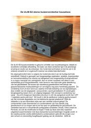
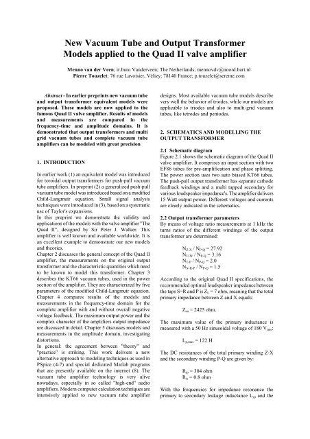
New Vacuum Tube and Output Transformer
Models applied to the Quad II valve amplifier
Menno van der Veen; ir.buro Vanderveen; The Netherlands; mennovdv@noord.bart.nl
Pierre Touzelet; 76 rue Lavoisier, Vélizy; 78140 France; p.touzelet@sereme.com
Abstract - In earlier preprints new vacuum tube
and output transformer equivalent models were
proposed. These models are now applied to the
famous Quad II valve amplifier. Results of models
and measurements are compared in the
frequency-time and amplitude domains. It is
demonstrated that output transformers and multi
grid vacuum tubes and complete vacuum tube
amplifiers can be modeled with great precision
1. INTRODUCTION
In earlier work (1) an equivalent model was introduced
for toroidal output transformers for push-pull vacuum
tube amplifiers. In preprint (2) a generalized push-pull
vacuum tube model was introduced based on a modified
Child-Langmuir equation. Small signal analysis
techniques were introduced in (3), based on a systematic
use of Taylor's expansions.
In this preprint we demonstrate the validity and
applications of the models with the valve amplifier "The
Quad II", designed by Sir Peter J. Walker. This
amplifier is well known and available worldwide. It is
an excellent example to demonstrate our new models
and theories.
Chapter 2 discusses the general concept of the Quad II
amplifier, the measurements on the original output
transformer and the characteristic quantities which need
to be known to model this transformer. Chapter 3
describes the KT66 vacuum tubes, used in the power
section of the amplifier. They are characterized by five
parameters of the modified Child-Langmuir equation.
Chapter 4 compares results of the models and
measurements in the frequency-time domain for the
complete amplifier with and without overall negative
voltage feedback. The maximum output power and the
complex character of the amplifiers output impedance
are discussed in detail. Chapter 5 discusses models and
measurements in the amplitude domain, investigating
distortions.
In general: the agreement between "theory" and
"practice" is striking. This work delivers a new
alternative approach to modeling techniques as used in
PSpice (4-7) and special dedicated Matlab programs
that are presently available on the internet (8). The
vacuum tube amplifier technology is very alive
nowadays, especially in so called "high-end" audio
amplifiers. Modern computer calculation techniques are
intensively applied to new vacuum tube amplifier
designs. Most available vacuum tube models describe
very well the behavior of triodes, while our models are
applicable to triodes and also to multi-grid vacuum
tubes, like tetrodes and pentodes.
2. SCHEMATICS AND MODELLING THE
OUTPUT TRANSFORMER
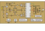
2.1 Schematic diagram
Figure 2.1 shows the schematic diagram of the Quad II
valve amplifier. It comprises an input section with two
EF86 tubes for pre-amplification and phase splitting.
The power section uses two auto biased KT66 tubes.
The push-pull output transformer has separate cathode
feedback windings and a multi tapped secondary for
various loudspeaker impedance's. The amplifier delivers
15 Watt output power. Different voltages and currents
are clearly indicated in the schematics.
2.2 Output transformer parameters
By means of voltage ratio measurements at 1 kHz the
turns ratios of the different windings of the output
transformer are determined:
NZ-X / NP-Q = 27.92
NU-W / NP-Q = 3.16
NT-P / NP-Q = 2.0
NS=R-P / NP-Q = 1.5
According to the original Quad II specifications, the
recommended optimal loudspeaker impedance between
the taps S=R and P is ZL = 7 ohm, meaning that the total
primary impedance between Z and X equals:
Zaa = 2425 ohm.
The maximum value of the primary inductance is
measured with a 50 Hz sinusoidal voltage of 180 Vrms:
Lp,max = 122 H
The DC resistances of the total primary winding Z-X
and the secondary winding P-Q are given by:
Rip = 304 ohm
Ris = 0.8 ohm
With the frequencies for impedance resonance the
primary to secondary leakage inductance Lsp and the

effective internal primary capacitance Cip are
determined:
Lsp = 6.4 mH
Cip = 467 pF
The parameters given above determine the behavior of
the output transformer in the frequency domain for a
speaker load of 7 ohm, as explained in full detail in (1).
3 MODELLING THE KT66
3.1 Handbook parameter set
Tube handbooks deliver information about the KT66.
The following set of data is used:
S = 6.3 mA/V
rp = 22.5 kohm
Ia0 = 85 mA
Ig20 = 6.3 mA
Vak0 = Vg20 = 250 V
Vg10 = -14.6 V
3.2 Five parameter set
According to the procedures as described in (2), the five
parameter set of the KT66 is calculated, resulting in:
[n ; αo ; K ; Da ; Dg2 ] =
[10 ; 0.966 ; 1.003·10 -3 ; 3.619·10 -3 ; 0.136]
The Child-Langmuir equation with its modification α
that belongs to the five parameter-set is given below:
I
α =
I
I
a
a
k
= α K
2
= [ Arctg (
V
α o
π V
( V
g1k
+ D
g2
V
g2k
ak
g2k
+ D
a
) ]
V
1/n
ak
)
3
2
(3.2.1)
3.3 Initial test of the new parameter set
A quick initial test is possible about the validity of the
equation 3.2.1 plus the five parameter set, by using the
voltages and currents in the quiescent operating point as
given in the schematic diagram of the Quad II amplifier.
The voltage at the cathode (tap V) equals Vk0 = 26 V.
Then Vak0 = 340 - 26 = 314 V and Vg2k0 = 330 - 26 =
304 V. The anode current equals Ia0 = 65 mA. With
formula 3.2.1 the control grid voltage Vg1k0 can be
calculated: Vg1k0 = -25,2 V, which only deviates 3% of
Vk0 = 26 V. Because [ Ik0 = Ia0 + Ig20 ] the calculated
screen grid current equals Ig20 = 7 mA as shown in the
diagram.
4 SMALL SIGNAL TRANSFER FUNCTION
4.1 Effective plate resistance of the KT66
Through the cathode windings at the output transformer
an amount Γ = NU-W / NZ-X = 0.11 of negative voltage
feedback is applied at the cathode of each KT66. In the
Quad II circuit there is no feedback at the screen grids,
so X = 0. Using the new coupling model of (2), the
effective plate resistance of each KT66 tube can be
calculated, resulting in:
rp,eff = 2 ri,eff = 1171 ohm
The total primary winding of the output transformer is
driven by two tubes. In (2) this circuit is represented by
a single voltage source with an effective generator
resistance Rgen,eff driving the total primary winding, with
Rgen,eff = 2 rp,eff = 2342 ohm
Again a quick initial test of this result is possible, by
calculating and measuring at 1 kHz the output
impedance Zout at the speaker terminals, when no
overall negative voltage feedback is applied (R11 is
temporally removed):
N
= [
N
2
] . ( R
+ R
) + R
Zout S-P
Z-X
gen, eff ip is
(4.1.1)
The calculated value of Zout equals 8.5 ohm, while the
measured value is 7.9 ohm (at 1 kHz sine wave and 2.8
Vrms at speaker terminals). These values differ 6.7%,
which is considered to be a negligible difference, taking
aging and deviations in specifications of tubes into
account.
Looking more precise into this, there appears to be
another effect. Using the Tailor expansions of (3), the
value of ri,eff can be calculated as function of the
alternating voltage at the control grids of the KT66
tubes. Figure 4.1 shows the result. At higher alternating
voltages the generator resistance becomes larger, which
easily can be explained considering the descending
slope of the Ia-Vak characteristics of the KT66 tube at
higher control grid voltages.
4.2 Transfer Function of power section
In (1) is explained how to calculate the transfer function
of the two KT66 tubes combined with the output
transformer. The primary inductance Lp,max of the
transformer, combined with the effective plate
resistance of the tubes create a first order high pass filter
with -3dB frequency f-3L:
f-3L = 1.55 Hz
At high frequencies Lsp and Cip create a second order
low pass filter with central frequency fo and Q-factor:
fo = 131 kHz
Q = 1 / a2 = 0.664

The normalized transfer function H1(f) of the KT66
tubes and the output transformer is shown in formula
4.2.1 (j = sqrt(-1)):
j.f
H 1(f)
=
j.f + f
-3L
.
1 +
1
Q
1
j.f
. + (
f
o
j.f
f
o
)
2
(4.2.1)
4.3 Transfer Function of the EF86 section
The input-driver section with the two EF86 tubes
contains two filters. The first is a high pass filter, first
order, created by the coupling capacitors C2 and C3
plus the resistors R7 and R9. Its -3dB frequency is
given by:
fC2,3-L = 1.85 Hz
The second filter is created by the 'large' output
impedance of the EF86 tubes and their 'large' anode
resistances R5 and R6, combined with the Miller
capacitance's at the control grids of the KT66 power
tubes. Its -3dB first order low pass frequency is given
by:
fEF86-H = 7.5 kHz
The normalized transfer function H2(f) of the EF86
section is given in formula 4.3.1.
j.f
H 2 (f) =
j.f + f
C2,3-L
f
.
j.f + f
EF86-H
EF86-H
(4.3.1)
4.4 Transfer Function of the complete amplifier
Without feedback in the amplifier (R11 temporally
removed) and without a loudspeaker connected to the
speaker terminals, the voltage amplification A0 at 1 kHz
is measured from input to output:
A0 = 100
The transfer function A0(f) of the total amplifier,
unloaded at the output, is given by formula 4.4.1 and
shown in the upper curve of figure 4.4.1:
(f) = A0
. H 1(f)
. H (f)
A0 2
(4.4.1)
With R11 connected, the effective feedback factor β
with respect to the 7 ohm tap S=R is given by:
β = NP-Q / NP-S R10 / (R10 + R11)
β = 0.117
The effective transfer function of the complete
amplifier, with negative voltage feedback and loaded by
a loudspeaker ZL is given by formula 4.4.2:
A
eff, L
A0
(f) Z L
(f) = .
1+
β . A0
(f) Z out
+ Z L
1+
β . A0
(f)
(4.4.2)
The two lower curves in figure 4.4.1 show the result of
the calculation with formula 4.4.2 and the measurement
with ZL = 7 ohm. The agreement is striking. Only at the
highest frequencies some partial resonance's appear in
the EI-core output transformer of the Quad II amplifier,
which are no part of the modeling of a toroidal core
output transformer in (1).
The calculated transfer at low frequencies with feedback
shows a maximum while the measurements show a
gentle roll off, see figure 4.4.1. This deviation can be
explained with the assumption that is made in the
calculation:
The frequency f-3L is calculated with the maximum
value LP,max. However, at small and moderate AC output
levels, the actual value of LP will be smaller (up to 10
times) than LP,max. Consequently f-3L will be larger than
the given value of 1.55 Hz. Implementing such a larger
f-3L value into the calculation causes the maximum to
disappear. Then measurements and calculation are in
full agreement again. See figure 4.4.2.
There is one peculiar condition where this maximum
can be noticed: "switch the amplifier off while listening
to music". Then the sound level will decrease 'swinging'
in loudness with a swing-frequency equal to the
frequency of the calculated maximum. But who listens
to an amplifier while switching the power off?
4.5 Output impedance
The output impedance Zout,eff of the complete amplifier
at a small signal output level is given by formula 4.4.3.
Z
out, eff
(f) =
1+
Z out
β . A
0
(f)
(4.4.3)
This formula shows that this output impedance is a
complex function, therefore |Zout,eff(f)| is shown in figure
4.5.
4.6 Voltages, Currents and Powers
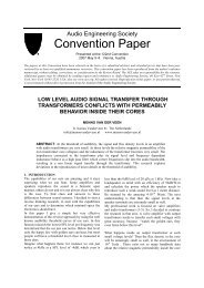
Figure 4.6.1 shows the calculated anode and screen grid
currents per KT66 tube as function of the momentary
anode voltage. With these data the output power Pout,
the anode dissipation Pa and the screen grid dissipation
Pg2 can be calculated as function of the alternating
control grid voltage. The results are shown in figure
4.6.2. The calculations show a maximum output power

of 18 W, while 15 W is measured. The difference can
be explained and calculated taking the transformer
winding resistances Rip and Ris into account, which
cause insertion loss inside the output transformer.
5 DISTORTIONS
5.1 Harmonic distortions without feedback
In (3) the procedure is explained how to calculate
harmonic distortions, using the Taylor expansions.
Figure 5.1 shows the results of the calculated distortions
at 1 kHz only in the section of KT66 tubes plus output
transformer. No overall feedback is applied nor any
influence of the EF86 vacuum tubes nor transformer
distortions are taken into account. It is striking that there
is no 2nd harmonic distortion, which is a direct
consequence of the push-pull concept.
5.2 Harmonic distortions with feedback
Applying overall negative feedback, the THD-figures of
figure 5.1 get smaller by the factor of 1 / (1+ βA0).
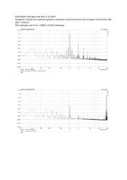
Figure 5.2 shows the calculated results plus measured
harmonic distortions at the actual amplifier.
The second harmonic distortion is not zero, as
calculated. The measured third harmonic distortion
appears to be 10 times larger than the calculated
distortion.
These deviations mainly are caused by not modeling the
EF86 circuitry nor taking output transformer behavior
into account.
The EF86 circuit can be modeled in the same way as the
KT66 vacuum tubes, however was not done in this
preprint.
The output transformer distortions are subject of present
research and modeling, taking the real dynamic B-H
relation of actual cores into account.
In general about distortions: only if the complete
amplifier is modeled, real calculations can be performed
with better precision. At this moment we are not ready
to show such results.
6 CONCLUSIONS
The output transformer of a push-pull vacuum tube
amplifier can be modeled with a simple equivalent
circuit as proposed in (1).
A multi grid vacuum tube can be modeled with the
modified Child-Langmuir equation as proposed in (2)
and (3). The model replaces the vacuum tubes in a
push-pull amplifier by an equivalent circuit, consisting
of a single voltage source with series generator
resistance. This resistance appears to be not constant
and depends on the momentary voltages at the tube.
The output impedance of a push-pull amplifier can be
calculated taking vacuum tube generator resistance and
output transformer specifications into account. There is
good agreement between calculations and measurement.
In the frequency domain the transfer function of
modeled tubes and output transformer can be calculated
with good precision. Only small partial high frequency
resonance's are not modeled.
The established theories of overall negative voltage
feedback are proven once again in this work.
The new vacuum tube and output transformer models
allow precise calculation of amplifiers output power,
power loss inside the output transformer, as well as heat
dissipations at screen grid and anode of each power
tube.
Harmonic distortions of a complete push-pull vacuum
tube amplifier can be calculated, although this
procedure has not yet been completed. Especially a new
model of the output transformer needs further work,
taking real B-H behavior inside the core into account.
It really is amazing, after so many years of the design
date of the Quad II amplifier (approx. 1950), to notice
that present computer modeling again proves the
excellent and sound qualities of this famous amplifier.
7 REFERENCES
1: Menno van der Veen: "Theory and Practice of Wide
Bandwidth Toroidal Output Transformers"; preprint
3887, AES convention 1994 November San Francisco
2: Menno van der Veen: "Modeling Power Tubes and
their Interaction with Output Transformers"; preprint
4643, AES convention 1998 May Amsterdam
3: Pierre Touzelet, Menno van der Veen: "Small Signal
Analysis for generalized push-pull tube amplifier
topology"; preprint 5587, AES convention 2002 May
Munich
4: W. Marshall Leach Jr.: "Spice models for
vacuum-tube amplifiers"; JAES Vol 43/3; 1995 March
5: Scott Reynolds: "Vacuum-tube models for Pspice
simulations"; Glass Audio; Vol 5/4 1993
6: Eric Pritchard: "Tube model critique"; Glass Audio;
Vol 8/1 1996
7: Norman Koren: "Improved Vacuum-tube models for
Spice simulations"; Glass Audio; Vol 8/5 1996
8: Eugene V. Karpov: good starting address for
internet search: www.next-power.net/next-tube.html

E ffective internal im pedance Ohm
700
650
600
550
Figure 2.1: Schematic Diagram of the Quad II Valve Amplifier
K T 66 - Vaà=314 Volt - Vg20=304 Volt - Vg10=-25,2 Volt - Z a=613 Ohm
500
0 10 20 30 40
Input signal e Volt
Figure 4.1: Effective impedance ri,eff as function of the alternating KT66 control grid voltage

Ao i
42
Aeff i
Am j
Ao i
0
42
Aeff i
0
20
Zeff i
0
40
20
0
40
20
.1 f i f 0.1 1 10 100 1 10
, , f
i j
3
Figure 4.4.1: Transfer functions in dB: upper curve is the calculation without NFB;
lower curves are measurements and calculation with NFB
10 6
1 10 6
0
0.1 1 10 100
.1 f , f
i i
100
Figure 4.4.2: Transfer function in dB: upper curve is calculation without NFB for Lp,max =12,2 H;
the lower curve is calculated with NFB.
20
10
0
.1 f 0.1 1 10 100 1 10
i
3
Figure 4.5: Effective output impedance (absolute value) of the amplifier with NFB for Lp = Lp,max.
1 10 4
1 10 4
1 10 5
1 10 5
10 6
1 10 6

Ia i
Ig2 i
Pa p
Figure 4.6.1: Anode current (upper curve) and Screen Grid Current (lower curve) per KT66
as function of the momentary anode voltage. The middle of the x-axis is the quiescent operating point.
30
Puit p
Pg2 p
.3
0
0 Va
i
0
0 p
2. Va0
Figure 4.6.2: Anode dissipation per KT66 (upper curve); output power (middle curve);
screen grid dissipation per KT66 (lower curve),
as function of the control grid voltage (arbitrary unit)
5

Harmonic distortion %
0,2
0,15
0,1
0,05
0
0 10 20
Input voltage e Volt
30 40
.2
T3m%
j
T3c% . 10
j
T2m% j
KT66 - Va0=314 Volt - Vg20=304 Volt - Vg10=-25,2 Volt - Za=613 Ohm
H2% H3% H4% H5%
Figure 5.1: Calculated harmonic distortions in KT66's plus OPT section
assuming no THD in the OPT and no NFB
0
0 ein
j
Figure 5.2: Harmonic Distortion (%) at 1kHz as function of the KT66 control grid voltage
with overall negative feedback:
2-nd harmonic distortion (measured, upper curve);
3-rd harmonic distortion (measured, 2-nd curve);
3-rd harmonic distortion times 10 (calculated, 3-rd curve).
30