Feynman Path Integrals in Quantum Mechanics

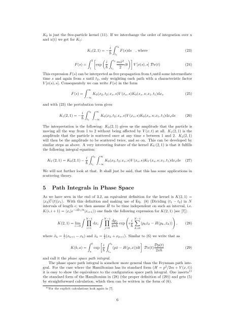
K 0 is just the free-particle kernel (11). If we interchange the order of integration over xand x(t) we get for K 1 :∫ t2K 1 (2, 1) = − ī F (s)ds , where (23)h t 1∫ 2[ ( ∫ īt2mẋ 2 )]F (s) = exp1 h t 12 dt V [x(s), s] Dx(t) (24)This expression F (s) can be interpreted as free propagation from t 1 until some intermediatetime s and again from s until t 2 , only weighting each path with a characteristic factorV [x(s), s]. Consequentely we can write F (s) in the formF (s) =∫ ∞−∞and with (23) the pertubation term givesK 1 (2, 1) = − ī h∫ t2∫ ∞t 1K 0 (x 2 , t 2 ; x s , s)V (x s , s)K 0 (x s , s; x 1 , t 1 )dx s (25)−∞K 0 (x 2 , t 2 ; x s , s)V (x s , s)K 0 (x s , s; x 1 , t 1 )dx s ds (26)The interpretation is the following: K 0 (2, 1) gives us the amplitude that the particle ismoving all the way from 1 to 2 without being affected by V (x, t) at all. K 1 (2, 1) is theamplitude that the particle is scattered once at any time s between 1 and 2. K 2 (2, 1)will then be the amplitude to be scattered twice, and so on. This can be developed bysimilar steps as above. A very interesting feature of the kernel K V (2, 1) is that it fulfillsthe following integral equation:K V (2, 1) = K 0 (2, 1) − ī h∫ t2∫ ∞t 1−∞K 0 (x 2 , t 2 ; x s , s)V (x s , s)K V (x s , s; x 1 , t 1 )dx s ds (27)We will not further look at that. It shall just be said, that this has some applications inscattering theory.5 Path Integrals in Phase SpaceAs we have seen in the end of 3.2, an equivalent definition for the kernel is K(2, 1) =〈x 2 |Û(t)|x 1〉. With this definition and making use of Eq. (8) (Dividing (t 1 − t 2 ) in Nintervals of length ɛ; we then assume Ĥ to be time independent on such an interval, i.e.K(i, i + 1) = 〈x i |e −iĤɛ/¯h |x i+1 〉) one finds the following expression for K(2, 1) [see [7]]:∫ N−1 ∏∫ N−1)∏ dp jK(2, 1) = lim dx i(ɛɛ→0 2π¯h exp ī N−1∑(p k ẋ k − H(p k , ¯x k )) , (28)hi=1 j=0k=0where ẋ k = 1 ɛ (x k+1 − x k ) and ¯x k = 1 2 (x k + x k+1 ). Similar to (6) we write that asK(b, a) =∫ ba[ īexph∫ tbt a](pẋ − H(p, x))dtDx(t) Dp(t)2π¯h(29)and call it the phase space path integral.The phase space path integral is somehow more general than the Feynman path integral.For the case where the Hamiltonian has its standard form (H = p 2 /2m + V (x, t))it is easy to show the equivalence to the configuration space path integral. One inserts 11the standard form of the Hamiltonian in (28) (the proper definition of (29)) and gets (5)by straightforward calculation, which then can be written in the form of (6).11 For the explicit calculations look again in [7].6