Ahmet Öztopal, Albero Mugnai, Daniele Casella, Marco ... - H-SAF

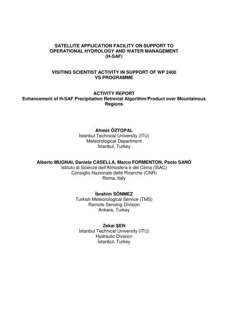
SATELLITE APPLICATION FACILITY ON SUPPORT TOOPERATIONAL HYDROLOGY AND WATER MANAGEMENT(H-SAF)VISITING SCIENTIST ACTIVITY IN SUPPORT OF WP 2400VS PROGRAMMEACTIVITY REPORTEnhancement of H-SAF Precipitation Retrevial Algorithm/Product over MountainousRegionsAhmet ÖZTOPALİstanbul Technical University (ITU)Meteorological Departmentİstanbul, TurkeyAlberto MUGNAI, Daniele CASELLA, Marco FORMENTON, Paolo SANÒIstituto di Scienze dell’Atmosfera e del Clima (ISAC)Consiglio Nazionale delle Ricerche (CNR)Roma, Italyİbrahim SÖNMEZTurkish Meteorological Service (TMS)Remote Sensing DivisionAnkara, TurkeyZekai ŞENİstanbul Technical University (ITU)Hydraulic Divisionİstanbul, Turkey

PREFACETurkey is a mountainous country which includes 4 different climate sturucture and due tothese special features, an enhanced Bayesian Algorithm is employed in the processingschedula of the project. This algorithm is developed based on Cloud-Radiation Database(CDR) from 14 rainy cases by Dr. Alberto MUGNAI and his team (Dr. Daniele CASELLA,Dr. Marco FORMENTON and Dr. Paolo SANÒ) from the Institute of AtmosphericSciences and Climate (ISAC) of the Italian National Research Council (CNR) work inEUMETSAT - Application Facility on Support to Operational Hydrology and WaterManagement (HSAF). Besides, Dr. İbrahim SÖNMEZ and Dr. Zekai ŞEN assisted in radarand raingauge data collection, assessment and validation. I would like to thank you all foryour valuable assistances, without which this report could not be completed successfully.Moreover, I would also like to thank Dr. Sante LAVIOLA, Dr. Vincenzo LEVIZZANI and Dr.Francesco Di PAOLA for their contributions.Dr. Ahmet ÖZTOPAL2

1. INTRODUCTIONIt is rather a very difficult task to determine ground rainfall amounts from fewSSMI/S channels. Although ground rainfall cannot be observed from the space directly, butknowledge about the cloud physics helps to estimate the amound of ground rainfall.SSMI/S includes so much information about the atmospheric structure, however it cannotprovide cloud micro-physical structural information. In such a situation, in the rainfallalgorithm, besides the SSMI/S data, it is necessary to incorporate cloud micro-physicalproperties from an external data source. These properties can be obtained quite simply bythe help of Cloud Resolving Model (CRM). Later, in addition to all available data, also microphysicalproperties obtained from Radiative Transfer Model (RTM) help to determine theSSMI/S brightness temperatures (Brightness temperatures – TBs), which can then becorrelated with Cloud-Radiation Database (CRD) data generation (Mugnai, et al., 2009).SSMI/S satellite data and CDR provide a common basis for rainfall predictionprocedure through CDR Bayesian probability algorithm, which combines the two sets ofdata in a scientific manner. The first applications of this algorithm, which is being used uptoday, is due to various researchers (Mugnai et al., 2001; Di Michele et al., 2003, 2005;Tassa et al., 2003, 2006)In this work, in order to establish a reflection of available data processing CDR CRMUniversity of Wisconsin – Non-hydrostatic Modeling System (UW-NMS) model isemployed, which is first developed by Prof. Gregory J. Tripoli (Tripoli, 1992; Tripoli andSmith,2008). It is also used by Turkish Meteorological Service by benefiting from radarnetwork data, and finally 14 simulations are realized in this study.2. STRUCTURE OF CLIMATE IN TURKEYTurkey is a mountainous contry located between warm and sub-tropical climateregions. Even though three sides are surrounded by seas. Mountain chain extensions andmorphology of Turkey, naturally, lead to various climate types within the country. Along thecoastal regions due to maritime effects warm climate types prevail, whereas continentalclimate type exists in the central regions, because of the Taurous ans Northern AnatolianMountains extensions as barrier from the coastal areas. According to Atalay (1997) andthe universal climate classification, the following climate types prevail in Turkey. Theseclimate regions are shown in Figure 2.1.1) Continental climate (a, b, c and d): Temperature differences between winterand summer seasons is rather high; precipitation takes place frequently in winter andspring seasons and during summer dry spells occur. Depending on the precipitation andtemperature features continental climate has four versions.2) Mediterranean Climate: Summersare hot and dry but in winters warmair withheavy precipitation exists. Hail and snow fall events are scarce along the coastal regions.However, at high elavations winters are snowy and cold.3) Marmara Climate: During winter, it is as hot as Mediterranean climate, but insummer not very rainy as much as Black Sea region. Winters are cold as conytinental3

climate and summers are hot and dry. Due to these features, Marmara climate has itsposition between continental Black Sea and Mediterranean Sea climates, as a transitionalzone.4) Black Sea Climate: Temperature differences between summer and winter arenot very significant. Summers are rather cool, winters at coastal areas are warm but withsnow and cold air at high elevation areas. Each season is rainy, and hence, there is notwater scarcity or stress.BLACK SEACONTINENTAL CLIMATEMEDITERRANEAN SEAMEDITERRANEAN CLIMATEMARMARA CLIMATEBLACK SEA CLIMATEFigure 2.1. Climate regions in Turkey3. OBSERVATION NETWORK IN TURKEYAs it is obvious in Figure 3.1, there are about 206 automatic stations in the westernpart of the country and they are within an the same obnservation network. The timeresolution of precipitation records at these station is almost 1 minute.Figure 3.1. Automated Weather Observation System (AWOS) station distribution inTurkey4

In total, there are four C Band Doppler radars and one of them has dual polarizationproperty (Figure 3.2). Among these, only İstanbul (a) and Balıkesir (b) located locationradars are adopted for in this study, but unfortunately, these they do not have dualpolarization property. In this work ,CAPPI product was used for radar data.abFigure 3.2. Radars and their coverage area in Turkey.4. METHODOLOGY4.1. Description of the Models4.1.1. Cloud Resolving Model (CRM)Time-dependent cloud/mesoscale numerical model with the three-dimensional (3-D)UW-NMS, is capable of simulating atmospheric phenomena with horizontal scales rangingfrom the microscale (turbulence) to the synoptic scale (extratropical cyclones, fronts, etc.).The non-Boussinesq quasi-compressible dynamical equations provide the basis on a setof assumptions as the model thermodynamics are based on the prediction of a moist iceliquidentropy variable, designed to be conservative over all ice and liquid adiabaticprocess (Tripoli and Cotton, 1981). Vorticity, kinetic energy and potential entrophy, whichare among the dynamic properties of flow are conserved by the advection scheme in theaforementioned model, which employs variable step topography. This approach is capableof capturing steep topographical slopes, and accurately represents subtle topographicvariations. Additionally, classical conservation equations are used for the specific humidityof total water and several ice and liquid water hydrometeor categories. A two-way multiplynested Arakawa “C” grid system modeling is the basis of the approach in this report, and itcast on a rotated spherical grid system, which includes multiple 2-way nesting capability.Such an approach helps to adjust locally enhanced resolutions in the most convenientway.The new version of UW-NMS includes microphysical module within H-SAF, which isa modified form of the scheme (Flatau et al., 1989; Cotton et al., 1986). Furthermore, the5

ice categories treatment and the precipitation physical specifications are different from theoriginal in the sense of performance enhancement. There are 6 hydrmeteor categories asfollows:1) Suspended cloud droplets,2) Precipitating rain drops,3) Suspended pristine ice crystals, and precipitation,4) Ice aggregates,5) Low-density graupel particles (or snow) and,6) High density graupel particles.In the application procedure, within the same grid volume at any given few or allthese categories may be used (for instance a couple of frozen and liquid hydrometeors) forthe hydrometeor category interaction.4.1.2. Radiative Transfer Model (RTM)It is necessary to include upwelling brightness temperatures (TBs) for simulationpurposes with the expectation of a radiative transfer (RT) code application to the simulatedprecipitation events’ microphysical outputs, which lead to the upwelling radiancescomputation based on the satellite footprints’ simulation. Such approaches cause heavycomputation overburden, because they are dependent on the cloud model simulation ofthe macrophysical structure. It is, therefore, for practical purposes, better to use simplermodels in one dimension, and hence, they are faster but have less accuracy. However, inthis study a 3-D adjusted plane parallel RT scheme is adopted as developed by Roberti etal. (1994) (see also Liu et al., 1996; Bauer et al., 1998; Tassa et al., 2003). The cloudmodel paths along the radiometer direction of sight help to generate the plane-parallelcloud structures rather then from the vertical cloud model columns. The RT approachalong a slanted profile in the direction of observation of the radiometer is employed withconfidence. One can observe that the downward flux is computed through the cloudstructure along the specular line that is reflected at the surface. It is observed that the usedmethod is computationally convenient and efficient. It also accounts for the geometricaland partially reducing errors in radiative transfer modelling. A genuine 3-D radiative effectsare not taken into consideration, due to the fact that the radiation is still trapped inside theslanted (and reflected) column. If there are enhanced horizontal inhomogeneities, then thesame approach may produce significant discrepancies with a fully 3D model outputs.Roberti et al., (1994) and Bauer et al., (1998) studied the performances of the slantedpathplane-parallel RT approximation and they agree on the error limitations concerning afew K on average scenes, Local values may be important in case of large horizontalgradients such as at the cloud edges (Liu et al., 1996; Czekala et al., 2000; Olson et al.,2001).After the completion of the monochromatic upwelling radiances at high resolution(i.e., at the resolution of the CRM model – 2 km) then the upwelling TBs at sensorresolution is computed for each channel through instrument transfer function. This isequivalent to the first integrating the monochromatic upwelling radiances over the channelwidth.It takes into account the channel spectral responsivity, and integrates the channelupwelling radiances over the field of view (i.e., over all cloud-model pixels that arecontained in the field of view) Finally, it also takes into account the radiometer antennapattern and radiometric noise. Subsequently, the high-resolution hydrometeor liquid/icewater content and the corresponding precipitation rate profiles for rain and ice areextracted from the cloud model simulations. They are then averaged over the field of viewin order to produce almost the same quantities at sensor resolution. The cloud structuredefinition is very important because it is associated with the simulated TBs. In genral, each6

channel has a different cloud structure. It fills up the slanted elliptical cylinder withcomparable sizes to the cross-track and along-track resolutions and it should beassociated with each TB point of the database. Such a strategy helps to make the multifrequencyretrieval rather complex and not univocal. It is, therefore, very convenient tochoose a common single resolution for the microphysical parameters that belong to thecloud-radiation database.CRM simulations outputs provide inputs for the radiative transfer model (RTM) forupwelling TBs generations, which are the vertical profiles of the liquid/ice water contents(LWC and IWC, respectively) of the various hydrometeors. Of course, they are alsocoupled with the surface temperature and the temperature/moisture profiles. Additionaloutputs are radiometer model, the surface emissivity model, and the single-scatteringmodel.Radiometer Model StructureIt provides a secondary input to the RT model. It also specifies all characteristics ofthe radiometer for simulation. Among the variables are the frequency, polarization andwidth of the candidate channels, view angle of the radiometer; field of view and antennapattern of the various channels. Instrument Transfer Function should be defined for eachchannel for the upwelling TBs computations from the upwelling monochromatic radiances.In this assessment, the following channel characteristics are important concerning theconically-scanning radiometers.1) Special Sensor Microwave Imager (SSM/I)2) Special Sensor Microwave Imager (SSMIS)3) TRMM Microwave Imager (TMI), and,4) Advanced Microwave Scanning Radiometer-EOS (AMSR-E)Surface Emissivity ModelsSurface emissivity impacts show themselves in the upwelling TBs more frequentlyat the lower frequencies as dependents on the frequency and polarization, observationgeometry, and surface characteristics (land/ocean, surface roughness, type of soil and soilcover, soil humidity, etc.). Three different surface emissivity models are selected for thepurpose of representing the different surface backgrounds of the selected CRMsimulations in the best possible manner. These surface emissivity models are as follows.1) The forest and agricultural land surface emissivity for land surfaces (Hewison,2001),2) The fast and accurate ocean emissivity model for a sea surface, (English andHewison, 1998; Hewison and English, 2000 and Schluessel et al, 1998). They provideaccurate surface emissivity estimations between 10 and 200 GHz for view angles up to60° and wind speeds from 0 to 20 m/s,3) The snow emissivity model that has been empirically derived for snow coveredsurfaces from satellite retrievals and ground-based measurements (Hewison, 1999). Fivedifferent snow cover types are considered for full range of snow emissivity. Such studiesare presented by some studies in the literature, such as the forest +snow, deep dry snow,fresh wet snow, frozen soil, first year ice, compact snow.Single-Scattering ModelsIt is a direct way to compute the single-scattering properties of the varioushydrometeor species in the cases of pure water and ice spheres only such as the Miescattering. However, it can be a major challenge for natural ice hydrometeors due to their7

wide variety of sizes, densities, and shapes. Information on shape is not available from theUW-NMS microphysical parameterization scheme, and therefore, for a successful study itis necessary to depend on a set of assumptions as folloows.1) Liquid (cloud and rain) particles have spherical forms, which are homogeneous,and accordingly their scattering properties can be computed by Mie theory (Bohren andHuffman, 1983). This approach necessitates the use of an efficient code as developed byWiscombe (1980).2) Graupel particles are in the form of spheres with densities almost equal to pureice (0.9 g cm-3) with “equivalent homogeneous spheres” and an effective dielectricprocedure combining the dielectric functions of ice and air (or water, in case of melting). Inthis it is carried out according to the effective medium Maxwell-Garnett mixing theory for atwo-component mixture of inclusions of air (water) in an ice matrix (Bohren and Huffman,1983).3) Pristine ice particles are highly non-spherical, and hence it is convenient to usethe Grenfell and Warren (1999) approximations (also Neshyba et al., 2003). The singlescatteringproperties of each nonspherical ice particle are computed by means of acollection of n s equal-size solid-ice spheres with a diameter, that is determined by thevolume, V, to cross-sectional area, A, ratio as V/A all of the original nonspherical iceparticle. The UW-NMS simulation outputs yield the volume values. On the other hand, thecross-sectional area comes through the observational relationship as A/(πD 2 /4) = C 0. Forseveral different individual particle habits D (in cm) is the maximum diameter of theparticle, while the coefficients C 0 and C (in appropriate cgs units) depend on ice particlehabit (Heymsfield and Miloshevich, 2003). For pristine ice crystals, C 0 = 0.18 and C =0.2707, that are indicated by the same authors as appropriate averages for midlatitude,continental mixed-habit cirrus clouds. It is possible to obtain the diameter, D s , and thenumber, n s , by the following formulations.DsρρD3+C0= nCs=3ice C0D1−C DsCDwhere, ρ ice = 0.916 g cm -3 while the density ρ of the pristine ice crystals is usually equal to0.1 g cm-3.It is well known that the snowflakes and ice aggregates have low-densities.Additionally, fluffy ice particles (as long as they are completely frozen) cannot be modelledaccording to Maxwell-Garnett mixing theory because “equivalent homogeneous soft-icespheres” would have, according to Mie theory, very large asymmetry factors (> 0.9) at thehigher microwave frequencies. Hence, it would not be adequately “cool” for the upwellingradiation. In order to overcome this problem, one can use the Surussavadee (2006) modelwhere non-spherical scattering results are fitted for spheres by Mie theory andcalculations with a density that is a function of the wavelength.4.2. Generation of the CRD Databases14 precipitation cases, which were observed between 2007 – 2009, are selected formaking CDR database (Table 4.1). These simulations are realized for red boxes in Figure4.1.8

Table 4.2. NMS model featuresNon-hydrostaticThree nested domains:• Domain 1, 50 Km resolution with 92 grid points• Domain 2, 10 Km resolution with 92 grid points• Domain 3, 2 Km resolution with 252 grid pointsFigure 4.2. Example of UW-NMS model rainfall rate in Domain 3.Figure 4.3. Example of UW-NMS total water (ice+liquid) in Domain 3.10

4.3. The CDRD Retrieval AlgorithmEspecially, Bayesian methodology helps to retrieve the precipitation indicators fromsatellite-borne microwave radiometers coupled with the Cloud Radiation Databases(CRDs) and they are composed of thousands of detailed microphysical cloud profiles.These are taken from Cloud Resolving Model (CRM) simulations, including thecorresponding brightness temperatures (TBs), which is calculated by applying radiativetransfer schemes to the CRM outputs. CRD’s play the role of generator for the CRMsimulations of past precipitation events. Subsequently, they can be used for the analysisof new events’ satellite observations.Figure 4.4 indicates the block diagram of our CDRD Bayesian algorithm, where thefollowing significant points must be taken into consideration for relevant interpretations(Sanò et al,2010).1) Prior to the estimation of TB measurements it is necessary to process the TBsmeasured by SSM/I or SSMIS (data processing block). This has to be done for eachchannel at the same geographical latitude and longitude position, Such interpolationprocedures are helpful for the low resolution channels.2) A “screening procedure” is employed for the data analysis for the decisionwhether to reject areas (pixels) either having incorrect TB values due to sensor errors orrecognized as areas without rain or with a very low probability of rain.3) The pixel selection is achieved by inversion algorithm, which uses a Bayesiandistance concept between the measured multi-frequency TB vector and all simulated multifrequencyTB vectors of the CDRD database.Figure 4.4. Block diagram of the CDRD Bayesian algorithm.11

5. ANALYSIS PROCEDURE5.1. StatisticsThere are 14 NMS simulations at high-resolution (2 km) profiles, which areassociated with TBs as averages to produce the sensor-resolution (15 km) profiles and thecorresponding TBs (SSM/I – SSMIS observation simulators). Table 5.1 includes thecomponents of each profile in the CRD database for SSM/I.Table 5.1. CRD database for SSM/I components of each profileTB19.35V (K) TB37.00H (K)TB19.35H (K) TB85.00V (K)TB22.24V (K) TB85.00H(K)TB37.00V (K)Vert-integrated cloud water path (kg/m**2)Vert-integrated rain water path (kg/m**2)vert-integrated graupel water path (kg/m**2)vert-integrated pristine water path (kg/m**2)vert-integrated snow water path (kg/m**2)vert-integrated aggregates water path (kg/m**2)Surface rain rate (mm/hr)Surface pristine (mm/hr )Surface aggregate (mm/hr )Surface graupel (mm/hr )Surface snow (mm/hr )Profile number Latitude LongitudePercent land Percent snow PercenticeHeight of surface (km)Iztop5.1.1. Microphysical QuantitiesSome simple but significant statistics of the cloud structure microphysical propertiesare presented in Table 5.2. Additionally, Figures 5.1 and 5.2 give the CRD Turkishdatabase. It is possible to sense that low water/ice contents and low precipitation are in themajority with a large variability in the cloud microphysical properties, which can be relatedto the coverage of different climatic regions, where types of precipitation and seasonalvariations occur in Turkey.Table 5.2. Statistics indexes of simulated TBs over land.Mean Variance SpreadCloud ColumnarContent (Kg m-2)Rain ColumnarContent (Kg m-2)Graupel ColumnarContent (Kg m-2)Pristine Ice ColumnarContent (Kg m-2)Snow ColumnarContent (Kg m-2)Aggregate ColumnarContent (Kg m-2)Surface Rain Rate(mm hr-1)0.25 0.13 0 – 4.370.30 0.67 1 - 29.950.07 0.28 0 – 40.150.62 1.87 0 – 18.010.34 0.40 0 – 4.800.04 0.02 0 – 4.660.97 10.85 1 – 184.6912

In Figure 5.1, it is worth to noticing that almost all are arount the peak value of 0 kg/m 2.Occourrence10.10.010.0010.0001Columnar contents pdfs0 1 2 3 4 5 6 7 8 9 10 11 12Cloud_ccRain_ccGraupel_ccPristine_ccSnow_ccAggregate_cc0.00001Figure 5.1. Probability Distribution Functions (PDFs) of the columnar contents (CC) ofliquid and frozen hydrometeors within the CRD Turkish database.Coupled with Table 5.2 it is obvious in Figure 5.2 that liquid precipitation have occasionallyvery high rates.10.1Rain rate pdfs0 10 20 30 40 50 60 70 80 90 100 110 120Occourrence0.010.0010.0001Rain rate0.00001Figure 5.2. PDFs of liquid precipitation rates at the surface within the CRD Turkishdatabase.5.1.2. Upwelling Brightness TemperaturesTables 5.3, 5.4 and 5.5 and Figures 5.3 to 5.5 provide the same statistics for thesimulated upwelling TBs for all relevant SSM/I – SSMIS channels within the CRDdatabase. Again, large variations may be observed, which are due to the wide range ofdifferent meteorological and environmental conditions of the simulated events.13

Table 5.3. Statistics indexes of simulated TBs over land.Over Land Polarization Mean Variance Spread ModeTB 19.35GHz V 273.77 48.99 226.41 - 292.82 274.60TB 19.35GHz H 271.11 147.04 189.75 - 292.82 276.45TB 22.235GHz V 274.85 22.36 237.15 - 291.19 276.12TB 37GHz V 273.84 21.32 195.08 - 292.07 274.29TB 37GHz H 272.85 43.99 195.07 - 292.07 274.29TB 85GHz V 271.07 72.02 99.42 - 291.48 272.08TB 85GHz H 270.85 74.59 99.41 - 291.48 275.28TB 91.66GHz V 271.03 78.62 98.78 - 291.57 273.02TB 91.66GHz H 270.82 80.89 98.78 - 291.57 273.51TB 150GHz V 269.09 126.47 93.26 - 287.91 271.24TB 150GHz H 269.02 126.67 93.26 - 287.91 272.72TB 183.31±7 H 262.93 67.97 94.12 - 278.73 264.23TB 183.31±3 H 254.80 33.73 96.81 - 269.99 251.61TB 183.31±1 H 243.50 20.41 110.96 - 259.34 239.63TB 50.3GHz H 268.99 21.21 155.88 - 285.25 268.62TB 52.8GHz H 258.14 7.55 174.75 - 269.66 258.35TB 53.596GHz H 244.13 3.97 190.95 - 252.56 244.35Table 5.4. Statistics indexes of simulated TBs over ocean.Over Ocean Polarization Mean Variance Spread ModeTB 19.35GHz V 208.65 181.99 182.57 - 264.07 199.27TB 19.35GHz H 156.52 575.36 107.53 - 257.43 130.62TB 22.235GHz V 231.01 143.48 199.38 - 270.92 227.58TB 37GHz V 227.88 122.89 164.96 - 263.24 219.62TB 37GHz H 182.92 595.75 134.29 - 257.54 155.14TB 85GHz V 258.14 193.96 61.22 - 279.07 261.01TB 85GHz H 239.28 330.94 61.22 - 273.21 235.06TB 91.66GHz V 259.60 214.89 61.15 - 280.95 263.47TB 91.66GHz H 242.44 318.68 61.15 - 273.66 234.39TB 150GHz V 265.15 371.46 69.23 - 285.82 270.59TB 150GHz H 261.73 341.08 69.23 - 283.93 267.94TB 183.31±7 H 260.26 259.16 75.08 - 277.95 263.17TB 183.31±3 H 253.14 145.28 79.42 - 271.85 255.99TB 183.31±1 H 242.71 67.05 91.12 - 261.73 239.46TB 50.3GHz H 240.2272 107.6749 122.17 - 265.50 238.52TB 52.8GHz H 254.4357 29.1565 140.14- 265.20 255.59TB 53.596GHz H 243.3057 10.6125 167.20 - 251.35 243.33Table 5.5. Statistics indexes of simulated TBs over coast.Over Coast Polarization Mean Variance Spread ModeTB 19.35GHz V 244.44 269.98 189.23 - 284.55 231.97TB 19.35GHz H 219.03 219.03 120.64 - 283.27 226.80TB 22.235GHz V 255.66 141.07 208.79 - 284.21 256.29TB 37GHz V 253.67 175.77 182.44 - 284.42 257.88TB 37GHz H 233.18 681.41 148.08 - 284.23 236.98TB 85GHz V 265.21 164.13 79.43 - 290.07 271.21TB 85GHz H 257.28 281.12 79.43 - 289.78 256.74TB 91.66GHz V 265.75 175.91 77.90 - 290.35 271.50TB 91.66GHz H 258.53 263.97 77.90 - 290.07 262.41TB 150GHz V 266.48 278.92 77.63 - 287.09 275.11TB 150GHz H 265.07 267.44 77.63 - 287.06 274.32TB 183.31±7 H 260.86 175.08 81.28 - 277.00 264.79TB 183.31±3 H 253.36 86.68 85.12 - 269.91 251.36TB 183.31±1 H 242.63 38.25 96.25 - 259.23 239.44TB 50.3GHz H 256.25 116.79 142.92 - 281.46 257.05TB 52.8GHz H 256.19 17.40 160.36 - 267.91 256.67TB 53.596GHz H 243.47 6.00 183.74 - 251.99 243.4614

A first glance on Figure 5.3 indicates first of all that there is a large difference between thePDF peaks for land and ocean, and it may be as a result of “cold” emission from the seasurface, which is coupled by land surfaces. Additionally, for each frequency there appearsa large difference over ocean between the two polarizations, and it may be due to thehigher ocean emissivity at vertical polarization.Low Frequency Channels pdfs Over Land0.14Occourrence0.120.10.080.060.040.020180 200 220 240 260 280 300Brightness Temperature (K)Ch 19.350 VCh 19.350 HCh 22.235 VCh 37.000 VCh 37.000 HLow Frequency Channels pdfs Over OceanOccourrence0.060.050.040.030.020.010100 120 140 160 180 200 220 240 260 280Brightness Temperature (K)Ch 19.350 VCh 19.350 HCh 22.235 VCh 37.000 VCh 37.000 HFigure 5.3. PDFs of the simulated upwelling TBs in the CRD / CDRD European databasefor the five low-frequency SSM/I – SSMIS window channels over land (top)and ocean (bottom).The graphs in Figure 5.4 indicate the differences between land and ocean as wellas the two polarizations, which are comparatively lower than for the low-frequencychannels. This is as a result of much larger atmospheric contribution to the upwelling TBs.15

High Frequency Channels pdfs Over LandOccourrence0.10.080.060.040.02040 60 80 100 120 140 160 180 200 220 240 260 280 300Brightness Temperature (K)Ch 91.660 VCh 91.660 HCh 150.000 VCh 150.000 HHigh Frequency Channels pdfs Over OceanOccourrence0.10.080.060.040.02040 60 80 100 120 140 160 180 200 220 240 260 280 300Brightness Temperature (K)Ch 91.660 VCh 91.660 HCh 150.000 VCh 150.000 HFigure 5.4. PDFs of the simulated upwelling TBs in the CRD / CDRD European databasefor the five high-frequency SSM/I – SSMIS window channels over land (top)and ocean (bottom).In Figure 5.5 there are two cases with corresponding results for the otherbackgrounds that are not shown herein. In the upper figure as a result of absorptionfrequencies there is much effective role in the atmosphere than the back-ground. Theprobability distribution function (PDF) peak position in each panel is colder for channelswith a peak weighting function at high atmospheric levels, whereas in the lower figurethere is a cold tail for the 183.31±7 channel. This is due to more external situation to theabsorption band because it is influenced more from ice scatter.16

Oxigen Band Channels pdfs Over LandOccourrence0.30.250.20.150.10.05060 80 100 120 140 160 180 200 220 240 260 280 300Brightness Temperature (K)Ch 50.300 HCh 52.800 HCh 53.596 HWater Vapour Band Channels pdfs Over OceanOccourrence0.160.140.120.10.080.060.040.02060 80 100 120 140 160 180 200 220 240 260 280 300Brightness Temperature (K)Ch 183.311 HCh 183.313 HCh 183.317 HFigure 5.5. PDFs of the simulated TBs for the three lower SSMIS channels in the 50-60GHz oxygen band over land (top) and for the three SSMIS channels in the 183GHz water vapor line over ocean (bottom).5.1.3. Comparison of Measured and Simulated Brightness TemperaturesIn this figure (Figure 5.6), different colors are employed for the indication of thedensity concerning two databases around each 19-37 GHz “point”. They are in terms ofthe log-occurrences at all 19-37 GHz couples as shown in the color bar. The simulationsdatabase are more consistent with the measurements apart from the long tail in thesimulations (especially at 19 GHz).17

Figure 5.6. 19.35 GHz vs. 37 GHz scatterplot of the simulated TBs in the Turkish CRDdatabase (top left) and of the measured TBs in the SSM/I – SSMISmeasurements database (top right) – in both case, over land only.Figure 5.7 represents in a better way than previous case as for the the consistencyof the simulations with the measurements. However, in Figure 5.6, 50.3 GHz is lesssensitive to surface characteristics than the lower window frequencies.Figure 5.7. 37 GHz vs. 50.3 GHz scatterplot of SSMIS simulated and measured TBs.Surface emissivity does not impact significantly on the upwelling TBs at these highwindow frequencies. However, exceptions are only in thin cloud presence with very lowprecipitation. On the other hand, the overall consistency for simulations database showsthe ice contents that are simulated rather properly by the UW-NMS model, where anappropriate ice scattering parameterizations is considered.18

Figure 5.8. 91.66 GHz vs. 150 GHz scatterplot of SSMIS simulated and measured TBs.Figure 5.9 presents intense water vapor line absorption frequencies at 183.31 GHz.Herein, the surface emissivity impact is negligible, but overall simulation consistencyshows the ice contents, which are simulated by the UW-NMS model. Accordingly,appropriate ice scattering parameterizations are adopted especially at higher cloudportions.Figure 5.9. 183.31±3 GHz vs. 183.31±7 GHz scatterplot of SSMIS simulated andmeasured TBs.5.2. Applications of the CDRD Algorithm5.2.1. Comparisions of Radar and RetrievalIn Figure 5.12a, scatter diagrams are obtained by considerations of 1x1 and 3x3resolution rain rate retrivals versus radar values, respectively. According to 45 degree line,the overall regression line indicates overestimation results with a very significant variability19

deviations in Figure 5.12a. This is tantamount to saying that there are undeterminism, andtherefore, one cannot depict the proper relationship between the two variables. In fact,there are many points that are zero for retrival values given a set of radar results. On theother hand, in Figure 12b, 3x3 spatial filtering is applied to available data, andconsequently, a better situation appeares, but still the retrivals have overestimations forearly data points.Rain Rate Radar (mm/hr)161412108642y = 0.3651x + 1.3246R 2 = 0.1831Rain Rate Radar (mm/hr)108642y = 0.5337x + 0.8952R 2 = 0.2726a00 2 4 6 8 10 12 14 16Rain Rate Retrieval (mm/hr)b00 2 4 6 8 10Rain Rate Retrieval (mm/hr)Figure 5.12. Scatter diagrams between radar and retrieval on 8 February 2009 at 05:41GMT (a) original comparision, (b) after applying a 3X3 filterThe following table (Table 5.6) provide the statistical values corresponding toscatter diagrams in Figure 5.12 with both filtering situations. Comparison of the statisticsfor both cases in the last two columns of the table shows naturally that the wider the filterarea the lower and more persistent are the parameters.Table 5.6. Statistical features (8 February 2009 at 05:41 GMT)Error Statistics 1X1 filter 3X3 filterMean Error 1.68 1.56Mean absolute error 2.94 2.13Mean squared error 14.64 6.41Root mean square error 3.83 2.53Standard deviation 3.44 2.02Correlation coefficient 0.43 0.52(Multiplicative) bias 1.55 1.42URD-RMSE 14.18 1.61So far as the rainfall occurrences are concerned, the following table (Table 5.7)includes different criteria that are already explained earlier during this project. It is obviousthat the rainfall occurrences are more pronounced in the case of 3x3 filtering case than thefiner resolution.Table 5.7. Rainfall occurrence indices (8 February 2009 at 05:41 GMT)Categorical Statistics 1X1 filter 3X3 filterPOD 0.82 1.00BIAS 0.87 1.00FAR 0.06 0.00CSI 0.77 1.00HR 0.80 1.00POFD 0.26 -99920

All what have been said about the two filtering cases are reflected in Figure 5.13 inthe form of spatial patches of rainfall occurrences and their quantities as shown in thecolor bars. It is obvious that the occurrence patterns are almost the same, but as for therainfall amounts are concerned, there are discrapencies. For instance, in the retrival case(Figure 5.13.a) although there are several sub-regions (peaks) with comparatively highrainfall amounts, radar case (Figure 5.13.b) has only a single peak.ab,,Figure 5.13. Patterns by using 3X3 filter on 8 February 2009 at 05:41 GMT (a) retrieval,(b ) radarFigure 5.14 is valid for 3 October 2008 at 05:44 GMT rainfall event both for retrivaland radar calculations. It is again obvious in Figure 5.15.a that there is a great scatter onthe basis of one-cell resolution and similarly overestimation still prevails, but comparedwith the case in Figure 5.13 the scatter are not very much concentrated on a certainportion on the Cartesian coordinate system. Comparison between the two cases indicatethat 3 October 2008 at 05:44 GMT event has less data points. On the other hand, coarserresolution (3x3 spatial filtering) yields better representation but still overestimation showsitself.Rain Rate Radar (mm/hr)3530252015105y = 0.7059x + 0.3093R 2 = 0.5026Rain Rate Radar (mm/hr)1512963y = 0.6038x + 0.2176R 2 = 0.8488a00 5 10 15 20 25 30 35Rain Rate Retrieval (mm/hr)b00 3 6 9 12 15Rain Rate Retrieval (mm/hr)Figure 5.14. Scatter diagrams between radar and retrieval on 3 October 2008 at 05:44GMT (a) original comparision, (b) after applying a 3X3 filter.21

The statistical properties of both resolution cases, namely, 1x1 and 3x3 spatialaverages are aailable in Table 5.8. Comparison of these statistics with the correspondingsin Table 5.6 indicates that 3 October 2008 at 05:44 GMT event has more stable behaviour.Table 5.8. Statistical features (3 October 2008 at 05:44 GMT)Error Statistics 1X1 filter 3X3 filterMean Error 0.07 0.26Mean absolute error 0.92 0.56Mean squared error 8.40 2.20Root mean square error 2.89 1.48Standard deviation 2.90 1.48Correlation coefficient 0.71 0.92(Multiplicative) bias 1.06 1.28URD-RMSE 4.85 0.95According to table 5.9 unfortunately rainfall occurrence cannot be even confirmedwith very high certainty in the case of 3 October 2008 at 05:44 GMT event than theprevious one.Table 5.9. Rainfall occurrence indices (3 October 2008 at 05:44 GMT)Categorical Statistics 1X1 filter 3X3 filterPOD 0.75 0.72BIAS 0.82 0.72FAR 0.08 0.00CSI 0.70 0.72HR 0.94 0.88POFD 0.02 0.00The rainfall spatial pattern in Figure 5.15 has a better match between retrieval andradar data especially in the form of two patches. Hence, areal coverage-wise, they aresimilar. Additionally, in the lower patch the rainfall amounts are also verbally correspondwith each other as low (high) rainfall points and in the retrieval pattern are in accordancewith low (high) radar patterns. However, numerically they are different especially at highrainfall areas.abFigure 5.15. Patterns by using 3X3 filter on 3 October 2008 at 05:44 GMT (a) retrieval,(b ) radar22

A third case study example is shown in Figure 5.16 concerning the radar andretrieval (model estimation data scatter diagrams correspondingly for 21 March 2008 at18:07 GMT. Both one-cell and 3-cell averaging (filtering) schemes have almost the samescatter on both Cartesian coordinate systems. In fact, it is very clear in Figure 5.16b thatthere is a non-linear relationship between the two sets of values. This is tantamount tosaying that the proposed model cannot depict the variation feature between the retrievaland radar measurements.25y = 0.4054x + 0.6505R 2 = 0.342410y = 0.5582x + 0.5549R 2 = 0.5655Rain Rate Radar (mm/hr)2015105Rain Rate Radar (mm/hr)8642a00 5 10 15 20 25Rain Rate Retrieval (mm/hr)b00 2 4 6 8 10Rain Rate Retrieval (mm/hr)Figure 5.16. Scatter diagrams between radar and retrieval on 21 March 2008 at 18:07GMT (a) original comparision, (b) after applying a 3X3 filter.Table 5.10 is for the statistical quantities and Table 5.11 is for categorical statistics.Both statistical quantities and categorical statistics are good.Table 5.10. Statistical features (21 March 2008 at 18:07 GMT)Statistics 1X1 filter 3X3 filterMean Error 0.51 0.23Mean absolute error 1.42 0.97Mean squared error 7.68 3.05Root mean square error 2.77 1.75Standard deviation 2.73 1.75Correlation coefficient 0.59 0.75(Multiplicative) bias 1.35 1.15URD-RMSE 13.63 59.24Table 5.11. Rainfall occurrence indices (21 March 2008 at 18:07 GMT)Categorical Statistics 1X1 filter 3X3 filterPOD 0.67 0.71BIAS 0.70 0.75FAR 0.05 0.05CSI 0.64 0.69HR 0.84 0.82POFD 0.03 0.0423

As the last example from rather mountainous area, Figure 5.17 depicts the spatialpattern on coarse and fine resolutions and again although they have similar arealcoverage, the rainfall amounts are not so close. After the comparison of all the threeprevious cases it is possible to state that the current model adjustment for any one ofthese cases may yield far better results, but then it will yield not so good results for othercases. Perhaps, what may be suggested is that the retrieval model approach should bedeveloped in such a manner to reduce the overall error from all the cases, this istantamount to saying that the sum of the squares of the errors must be minimized.abFigure 5.17. Patterns by using 3X3 filter on 21 March 2008 at 18:07 GMT (a) retrieval,(b) radar9 September 2009 at 03:40 GMT case yields scatter diagrams as in Figure 5.18 andit has rather similar case to Figure 5.16, in the sense that the regression relationship isvery close to linear and not as in Figure 5.17 non-linear.Rain Rate Radar (mm/hr)70605040302010y = 0.2904x + 0.814R 2 = 0.3022Rain Rate Radar (mm/hr)3530252015105y = 0.3313x + 0.4336R 2 = 0.6763a00 10 20 30 40 50 60 70Rain Rate Retrieval (mm/hr)00 5 10 15 20 25 30 35Rain Rate Retrieval (mm/hr)Figure 5.18. Scatter diagrams between radar and retrieval on 9 September 2009 at 03:40GMT (a) original comparision, (b) after applying a 3X3 filterb24

Table 5.12 is for the statistical quantities and Table 5.13 is for categorical statistics.Both statistical quantities and categorical statistics are very good.Table 5.12. Statistical features (9 September 2009 at 03:40 GMT)Statistics 1X1 filter 3X3 filterMean Error 2.51 3.15Mean absolute error 3.44 3.34Mean squared error 63.49 40.57Root mean square error 7.97 6.37Standard deviation 7.57 5.64Correlation coefficient 0.55 0.87(Multiplicative) bias 2.15 2.25URD-RMSE 15.78 21.08Table 5.13. Rainfall occurrence indices (9 September 2009 at 03:40 GMT)Categorical Statistics 1X1 filter 3X3 filterPOD 0.86 0.90BIAS 0.99 0.90FAR 0.13 0.00CSI 0.77 0.90HR 0.89 0.93POFD 0.08 0.00All the three previous rainfall events are from rather mountainous area, andtherefore, the scatters cannot be accounted on the basis of atmospheric phenomena only,but also surface features in the form of morphology must also be considered. In order tocheck whether there is an effect of rugged area compared to rather flat surfaces, in Figure5.19 comparatively flat area of İstanbul and its vicinity is adopted with the retrieval as wellas radar patterns, separately. It is very interesting after the comparison of this figure withall three figures (Figures 5.16, 5.17 and 5.18) to depict that the retrieval and radar patternshave almost the same regional shape and also the quantitative rainfall values are ratherclose to each other.abFigure 5.19. Patterns by using 3X3 filter on 9 September 2009 at 03:40 GMT (a) retrieval,(b ) radar25

5.2.2. Validation of Retrieval by using RaingaugeIn this work H01 based on SSMI/S and H02 based on AMSU are used for validationby using raingauge. Turkish CDR database and Bayasien Algorithm for H01 and NEXRADversion of AMSU algorithm are used. All statistics are given in Tables 5.6 and 5.7.Moreover, common validation methodology in HSAF is applied to this research forvalidation.Table 5.6. Summary results of PR-OBS-1 validation in Turkey over inner landLan Validation period: 1 st July 2008 - 30 June 2009 - Threshold rain / no rain:H01 Turkeyd0.25 mm/hGauge Class Jul Aug Sep Oct Nov Dec Jan Feb Mar Apr May JunNumber of > 10 mm/h 0 12 196 17 45 0 12 0 0 1 0 44comparison1-10 mm/h 1671 744 13426 5370 8119 7499 15882 18603 7626 9459 7527 4717s(ground< 1 mm/h 3246 1232 25065 15474 21879 32645 36493 46103 35365 28461 21365 10435obs.)> 10 mm/h - -10.66 -13.04 -12.60 -10.83 - -2.66 - - -10.13 - -5.76ME (mm/h) 1-10 mm/h -0.97 -4.27 -0.48 -0.71 -0.66 -0.33 -0.21 -0.18 -0.11 1.19 1.97 0.99< 1 mm/h -0.14 0.24 0.16 0.11 -0.17 -0.06 -0.01 -0.01 -0.01 0.36 1.22 1.01> 10 mm/h - 0.38 5.59 2.86 3.41 - 16.61 - - - - 9.10SD (mm/h) 1-10 mm/h 3.38 2.60 4.12 3.48 3.59 3.29 4.31 3.23 3.79 5.18 6.44 6.53< 1 mm/h 1.56 2.98 2.42 2.18 1.46 1.88 2.03 1.94 1.88 2.56 4.58 4.26RMSE(mm/h)> 10 mm/h - 10.67 14.18 12.91 11.35 - 16.12 - - 10.13 -1-10 mm/h 3.51 5.00 4.14 3.55 3.65 3.31 4.31 3.24 3.80 5.32 6.74 6.61< 1 mm/h 1.57 2.99 2.42 2.19 1.47 1.89 2.03 1.94 1.88 2.58 4.74 4.38> 10 mm/h - 100 94 99 93 - 145 - - 100 - 100RMSE (%) 1-10 mm/h 228 142 230 209 187 197 220 214 228 311 431 403< 1 mm/h 293 553 597 440 323 456 416 409 419 504 992 830> 10 mm/h - - 0.15 -0.18 -0.09 - -0.12 - - - - -0.20CC 1-10 mm/h -0.02 -0.22 0.05 0.04 0.11 0.32 0.20 0.13 0.21 0.18 0.16 0.03< 1 mm/h 0.15 0.30 0.02 0.08 0.06 0.04 0.08 0.08 0.09 0.15 0.13 0.18POD ≥ 0.25 mm/h 0.15 0.09 0.19 0.15 0.01 0.10 0.12 0.13 0.11 0.22 0.35 0.34FAR ≥ 0.25 mm/h 0.83 0.93 0.53 0.69 0.68 0.84 0.83 0.71 0.83 0.51 0.56 0.63CSI ≥ 0.25 mm/h 0.09 0.04 0.16 0.12 0.08 0.06 0.07 0.10 0.07 0.18 0.24 0.2210.6926

Table 5.7. Summary results of PR-OBS-2 validation in Turkey over inner landH02 Turkey LandValidation period: 1 st July 2008 - 30 June 2009 - Threshold rain / no rain: 0.25mm/hGauge Class Jul Aug Sep Oct Nov Dec Jan Feb Mar Apr May JunNumber of > 10 mm/h 0 0 3 - 5 0 0 1 0 18 - 9comparisons1-10 mm/h 452 352 2864 - 2472 1800 6126 6763 3395 3464 - 1620(groundobs.)< 1 mm/h 1052 581 6515 - 7470 7961 14274 18339 12536 9413 - 3147> 10 mm/h - - -12.65 - -10.39 - - -12.39 - -12.40 - -3.22ME (mm/h) 1-10 mm/h 3.20 13.47 -0.81 - -1.63 -1.27 -1.38 -1.46 -1.28 -1.08 - 0.78< 1 mm/h 2.29 3.19 0.22 - -0.46 -0.44 -0.47 -0.46 -0.48 -0.33 - 1.38> 10 mm/h - - 0.78 - 2.05 - - - - 3.58 - 24.29SD (mm/h) 1-10 mm/h 17.64 30.55 4.20 - 1.35 0.77 1.26 0.83 1.04 1.85 - 9.04< 1 mm/h 11.57 15.71 5.05 - 0.35 0.34 0.37 0.50 0.37 0.81 - 6.73> 10 mm/h - - 12.67 - 10.55 - - 12.39 - 12.87 - 23.13RMSE(mm/h)1-10 mm/h 17.91 33.34 4.27 - 2.12 1.48 1.87 1.68 1.65 2.14 - 9.07< 1 mm/h 11.79 16.02 5.05 - 0.58 0.56 0.60 0.68 0.60 0.88 - 6.87> 10 mm/h - - 100 - 94 - - 100 - 89 - 166RMSE (%) 1-10 mm/h 1094 2055 254 - 97 96 97 94 104 106 - 531< 1 mm/h 2918 2406 1349 - 108 108 112 121 108 180 - 1642> 10 mm/h - - - - -0.23 - - - - 0.03 - -0.29CC 1-10 mm/h 0.23 0.11 0.03 - 0.30 0.16 0.36 0.21 0.16 0.26 - 0.00< 1 mm/h -0.02 0.24 -0.01 - 0.11 0.08 0.08 0.05 0.10 0.07 - 0.05POD ≥ 0.25 mm/h 0.11 0.21 0.13 - 0.08 0.06 0.10 0.09 0.06 0.14 - 0.21FAR ≥ 0.25 mm/h 0.55 0.61 0.43 - 0.23 0.33 0.37 0.26 0.36 0.31 - 0.64CSI ≥ 0.25 mm/h 0.10 0.15 0.12 - 0.08 0.06 0.09 0.09 0.05 0.14 - 0.15Values in Table 5.6 and Table 5.7 are presented in graphical form in Figure 5.20 andFigure 5.21, respectively. As for Figure 5.20 the following interpretation sequence can bedrawn.1) It is clear from Figure 5.20a that the standard deviation (SD) and root Mean squareerror (RMSE) have almost the same pattern, and therefore, in the future onlyRMSE must be considered.2) RMSE variation for < 1 mm/h precipitation is comparatively smaller that the otheralternative where the precipitation amounts lie within 1 mm/h and 10 mm/h interval.This is meaningful because extreme precipitation fluctuations are within this intervaland also the number of precipitation occurrences in this interval is less than theoccurrences, where precipitation is < 1mm/h.3) The mean error (ME) values fluctuate around zero level for the case whereprecipitation is < 1mm/h, which indicates the suitability of the used model.4) Unfortunately, the ME values for 1-10 mm/h interval have dominantly negatives,which means that the model yields biased results. However, since all the valuesfluctuate around almost -1.0 level it is possible to improve the model by introducinga constant value, which helps to shift -1.00 level to zero level.5) In Figure 5.20b there are significant errors because precipitation category morethan 10 mm/h includes very extreme values and accordingly their treatments mustbe dealt with a separate approach and model.27

6) It is very obvious in Figure 5.20c that as the category values increase (from < 1mm/h, to 1-10 mm/h, then to > 10 mm/h) so does the irregularity behaviour of thecorrelation coefficient. Although, there are not significant outlier appearance in < 1mm/h correlation coefficient, for 1-10 mm/h the maximum correlation is in almostDecember7) In Figure 5.20d FAR is usually high and CSI is very low.Figure 5.21 graphs lead to the following sequence of interpretations.1) In Figure 5.21a ME, SD and RMSE are parallel to each other. ME is negative for< 1.0 mm/hr and 1-10 mm/hr precipitation between November 2008 and April2009. Other statistics are positive and low for this time interval. On the otherhand, all statistic scores are high between July and September 2008 than othersmonths.2) Figure 5.21b includes very extreme case (> 10 mm/h) ME, SD and RMSEvalues, where again the ME has all negative values but all of them are around ahorizontal line.3) Figure 5.21c represents the correlation coefficient variation with time and as thecategory increases the correlation coefficient variation becomes morehaphazard.4) POD and CSI values are very low in Figure 5.21.d.28

Mean Error, Standart Deviation and RMSE for H01 (Land)Scoresa86420-2-4Jul2008Aug Sep Oct Nov Dec Jan2009MonthsFeb Mar Apr May JunME 1 - 10 mm/hME < 1 mm/hSD 1 - 10 mm/hSD < 1 mm/hRMSE 1 - 10 mm/hRMSE < 1 mm/hMean Error, Standart Deviation and RMSE for H01 (Land)Scoresb20151050-5-10Jul 2008-15AugSepOctNovDecJan 2009FebMonthsMarAprMayJunME > 10 mm/hSD > 10 mm/hRMSE > 10 mm/hCorrelation Coefficients For H01 (Land)0.40.3Scoresc0.20.10-0.1-0.2Jul 2008-0.3AugSepOctNovDecJan 2009MonthsFebMarAprMayJun> 10 mm/h1 - 10 mm/h< 1 mm/hScoresd10.80.60.40.20Jul 2008AugSepMulti-Categorical Scores for H01 (Land)OctNovDecJan 2009MonthsFigure 5.20. Continuous and multi-categorical statistics for inner land.FebMarAprMayJunPOD ≥ 0.25 mm/hFAR ≥ 0.25 mm/hCSI ≥ 0.25 mm/h29

Mean Error, Standart Deviation and RMSE for H02 (Land)40Scoresa3020100-10Jul 2008AugSepOctNovDecJan 2009MonthsFebMarAprMayJunME 1 - 10 mm/hME < 1 mm/hSD 1 - 10 mm/hSD < 1 mm/hRMSE 1 - 10 mm/hRMSE < 1 mm/hMean Error, Standart Deviation and RMSE for H02 (Land)3020Scoresb100-10Jul 2008-20AugSepOctNovDecJan 2009MonthsFebMarAprMayJunME > 10 mm/hSD > 10 mm/hRMSE > 10 mm/hCorrelation Coefficients For H02 (Land)Scoresc0.40.30.20.10-0.1-0.2-0.3-0.4Jul 2008AugSepOctNovDecJan 2009MonthsFebMarAprMayJun> 10 mm/h1 - 10 mm/h< 1 mm/hMulti-Categorical Scores for H02 (Land)Scoresd0.80.60.40.20Jul 2008AugSepOctNovDecJan 2009MonthsFebMarAprMayFigure 5.21. Continuous and multi-categorical statistics for inner land.JunPOD ≥ 0.25 mm/hFAR ≥ 0.25 mm/hCSI ≥ 0.25 mm/h30

6. SUMMARY AND CONCLUSIONIn this study, for PR-OBS-1 (Precipitation Rate at Ground by MW Conical Scanners)a Turkish databese is structured and with these data the Bayesian approached isebhanced by all means. The rainfall products through such a study is validated by TurkishCDR on 206 rainfall stations within the same network and with 2 single polarization C banddoppler radars. Additionally, NEXRAD version of PR-OBS-2 (Precipitation rate at groundby MW cross-track scanners) is aso taken into consideration during the validation process.As already defined earlier in this report four rainfall events in radar on 8 February2009, 3 October 2008, 21 March 2008 and 9 September 2009 are compared with retrievalvalues and in all the cases overestimations are observed. Especially at brathermountainous region of Balıkesir it is observed that coarser resolution (3x3 filter) indicatessome improvements compared to fşner filter cases. However, on 9 September 2009rainfall event on comparatively flat area matches far better with the retrieval values andhence the spatial rainfall occurrence extent and numerical values are very close to eachother than any other three cases in Balıkesir.As a conclusion one can conclude that the retrieval yields overestimations. At thispoint due to the single polarization of radars lower values might be obtained aso and thispoint must be taken into consideration in the future studies. Apart from all these, thecoverage area of the radar will also help to improve the results, because in themountainous areas there are blockage effects due to high hills.PR-OBS-1 ve PR-OBS-2 products are rather low POD and CSI values comparedwith the validation results during July-August-2009 period, but FAR values are high.Along with the results that emerge from this study it is adviced to try and improvethe efficiency of the algorithm in the future.31

7. REFERENCESBauer, P., L. Schanz and L. Roberti, 1998: Correction of the three-dimensional effects forpassive microwave remote sensing of convective clouds. J. Appl. Meteor., 37, 1619-1632.Bohren, C.F., and D.R. Huffman, 1983: Absorption and Scattering of Light by Smal particles.John Wiley & Sons, 530 pp.Cotton, W.R., G.J. Tripoli, R.M. Rauber and E.A. Mulvihill, 1986: Numerical simulation of theeffects of varying ice crystal nucleation rate and aggregation processes on orographicsnowfall. J. Clim. Apl. Meteor. 25: 1658-1680.Czekala, H., P. Bauer, D. Jones, F. Marzano, A. Tassa, L. Roberti, S. English, J.P.V. PoiaresBaptista, A. Mugnai and C. Simmer, 2000: Clouds and Precipitation. Radiative TransferModels for Microwave Radiometry (C. Matzler, Ed.), COST Action 712, Directorate-General for Research, European Commission, Brussels, Belgium, 37-72.Di Michele S., A. Tassa, A. Mugnai, F.S. Marzano, P. Bauer and J.P.V. Poiares Baptista,2005: The Bayesian Algorithm for Microwave-based Precipitation Retrieval: Descriptionand application to TMI measurements over ocean. IEEE Trans. Geosci. Remote Sens.,43, 778-791.Di Michele S., F.S. Marzano, A. Mugnai, A. Tassa and J.P.V. Poiares Baptista, 2003:Physically-based statistical integration of TRMM microwave measurements forprecipitation profiling. Radio Sci., 38, 8072-8088.English, S.J., and T.J. Hewison, 1998: A fast generic millimetre wave emissivity model. Proc.SPIE on Microwave Remote Sensing of the Atmosphere and Environment, 22- 30.Flatau P., G.J. Tripoli, J. Berlinde and W. Cotton, 1989: The CSU RAMS Cloud MicrophysicsModule: General Theory and Code Documentation. Technical Report 451, ColoradoState University, 88 pp.Grenfell, T.C., and S.G. Warren, 1999: Representation of a nonspherical ice particle by acollection of independent spheres for scattering and absorption of radiation. J.Geophys. Res., 104, 31697-31709.Hewison, T.J., 2001: Airborne measurements of forest and agricultural land surface emissivityat millimeter wavelengths. IEEE Trans. Geosci. Remote Sens., 39, 393-400.Hewison, T.J., and S.J. English, 1999: Airborne retrievals of snow and ice surface emissivity atmillimetre wavelengths. IEEE Trans. Geosci. Remote Sens., 37, 1871-1879.Hewison, T.J., and S.J. English, 2000: Fast models for land surface emissivity. RadiativeTransfer Models for Microwave Radiometry (C. Matzler, Ed.), COST Action 712,Directorate- General for Research, European Commission, Brussels, Belgium, 117-127.Liu, G., C. Simmer and E. Ruprecht, 1996: Three-dimensional radiative transfer effects ofclouds in the microwave spectral range. J. Geophys. Res., 101, 4289-4298.Mugnai, A., Casella, D., Formenton, M., Sanò, P., Tripoli, G. J., Leung, W. L., Smith, E. A.,Mehta, A., 2009, Generation of an European Cloud-Radiation Database to be usedfor PR-OBS-1 (Precipitation Rate at Ground by MW Conical Scanners), ActivityReport, EUMETSAT – HSAF Project, 39 pp.Mugnai, A., S. Di Michele, F.S. Marzano and A. Tassa, 2001: Cloud-model based Bayesiantechniques for precipitation profile retrieval from TRMM microwave sensors.ECMWF/EuroTRMM Workshop on Assimilation of Clouds and Precipitation, ECMWF,Reading, U.K., 323-345.Neshyba, S.P., T.C. Grenfell and S.G. Warren, 2003: Representation of a nonspherical iceparticle by a collection of independent spheres for scattering and absorption ofradiation: 2. Hexagonal columns and plates. J. Geophys. Res., 108, 4448-4465.32

Olson, W.S., P. Bauer, N.F. Viltard, D.E. Johnson, W.K. Tao, R. Meneghini and L. Liao, 2001:A melting layer model for passive/active microwave remote sensing applications. PartII: Simulation of TRMM observations. J. Appl. Meteor., 40, 1164-1179.Roberti, L., J. Haferman and C. Kummerow, 1994: Microwave radiative transfer throughhorizontally inhomogeneous precipitating clouds. J. Geophys. Res., 99, 707-716.Sanò, P., D. Casella, S. Dietrich, F. Di Paola, M. Formenton, W.-Y. Leung, A. Mehta, A.Mugnai, E.A. Smith and G.J. Tripoli, 2010: Bayesian estimation of precipitation fromspace using the Cloud Dynamics and Radiation Database (CDRD) approach:Application to case studies of FLASH and H-SAF Projects. Nat. Hazards Earth SystSci., to be submitted.Schluessel, P.; and H. Luthardt, 1998: Surface wind speeds over the North Sea from SpecialSensor Microwave/Imager observations. J. Geophys. Res., 96, 4845–4853.Surussavadee, C., 2006: Passive millimeter-wave retrieval of global precipitation utilizingsatellites and a numerical weather prediction model. Ph.D. dissertation, Dept. Elect.Eng. and Comput. Sci., MIT, Cambridge, MA.Tassa, A., S. Di Michele, A. Mugnai, F.S. Marzano, P. Bauer and J.P.V. Poiares Baptista,2006: Modeling uncertainties for passive microwave precipitation retrieval: Evaluationof a case study. IEEE Trans. Geosci Remote Sens., 44, 78-89.Tassa, A., S. Di Michele, A. Mugnai, FS. Marzano and J.P.V. Poiares Baptista, 2003: Cloudmodelbased Bayesian technique for precipitation profile retrieval from the TropicalRainfall Measuring Mission Microwave Imager. Radio Sci., 38, 8074-8086.Tripoli G.J. and E.A. Smith, 2009: Scalable nonhydrostatic cloud/mesoscale model featuringvariable-stepped topography coordinates: Formulation and performance on classicobstacle flow problems. Mon. Wea. Rev., submitted.Tripoli, G.J., 1992: A nonhydrostatic model designed to simulate scale interaction. Mon. Wea.Rev., 120, 1342-1359.Tripoli, G.J., and W.R. Cotton, 1981: The use of ice-liquid water potential temperature as athermodynamic variable in deep atmospheric models. Mon. Wea. Rev., 109, 1094-1102.Wiscombe, W.J., 1980: Improved Mie scattering algorithms. Appl. Opt., 19, 1505-1509.33