Modeling and Optimization of Traffic Flow in Urban Areas - Czech ...

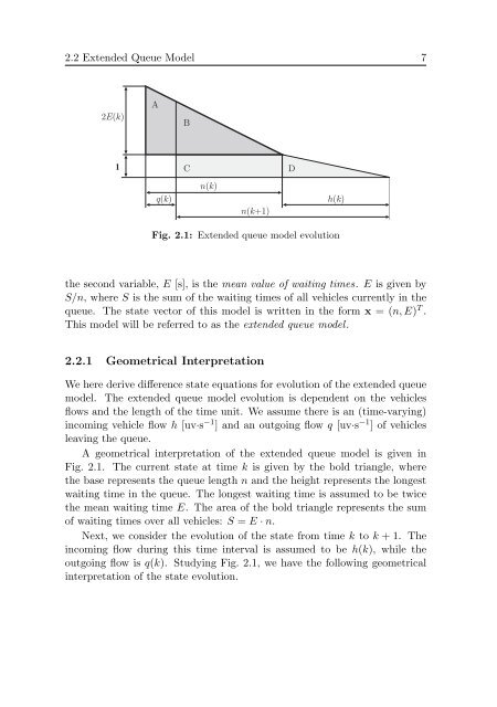
2.2 Extended Queue Model 72 E( k)AB1CDq( k)n( k)n( k+1)h( k)Fig. 2.1: Extended queue model evolutionthe second variable, E [s], is the mean value of waiting times. E is given byS/n, where S is the sum of the waiting times of all vehicles currently in thequeue. The state vector of this model is written in the form x = (n, E) T .This model will be referred to as the extended queue model.2.2.1 Geometrical InterpretationWe here derive difference state equations for evolution of the extended queuemodel. The extended queue model evolution is dependent on the vehiclesflows and the length of the time unit. We assume there is an (time-varying)incoming vehicle flow h [uv·s −1 ] and an outgoing flow q [uv·s −1 ] of vehiclesleaving the queue.A geometrical interpretation of the extended queue model is given inFig. 2.1. The current state at time k is given by the bold triangle, wherethe base represents the queue length n and the height represents the longestwaiting time in the queue. The longest waiting time is assumed to be twicethe mean waiting time E. The area of the bold triangle represents the sumof waiting times over all vehicles: S = E · n.Next, we consider the evolution of the state from time k to k + 1. Theincoming flow during this time interval is assumed to be h(k), while theoutgoing flow is q(k). Studying Fig. 2.1, we have the following geometricalinterpretation of the state evolution.