Modeling and Optimization of Traffic Flow in Urban Areas - Czech ...

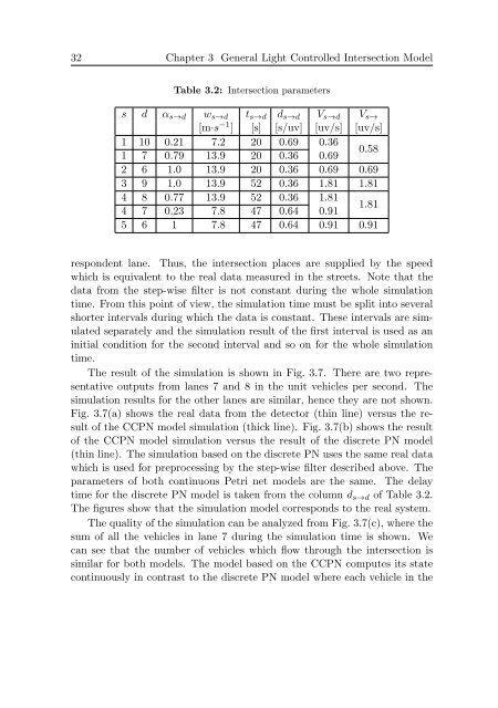
32 Chapter 3 General Light Controlled Intersection ModelTable 3.2: Intersection parameterss d α s→d w s→d t s→d d s→d V s→d V s→[m·s −1 ] [s] [s/uv] [uv/s] [uv/s]1 10 0.21 7.2 20 0.69 0.361 7 0.79 13.9 20 0.36 0.690.582 6 1.0 13.9 20 0.36 0.69 0.693 9 1.0 13.9 52 0.36 1.81 1.814 8 0.77 13.9 52 0.36 1.814 7 0.23 7.8 47 0.64 0.911.815 6 1 7.8 47 0.64 0.91 0.91respondent lane. Thus, the intersection places are supplied by the speedwhich is equivalent to the real data measured in the streets. Note that thedata from the step-wise filter is not constant during the whole simulationtime. From this point of view, the simulation time must be split into severalshorter intervals during which the data is constant. These intervals are simulatedseparately and the simulation result of the first interval is used as aninitial condition for the second interval and so on for the whole simulationtime.The result of the simulation is shown in Fig. 3.7. There are two representativeoutputs from lanes 7 and 8 in the unit vehicles per second. Thesimulation results for the other lanes are similar, hence they are not shown.Fig. 3.7(a) shows the real data from the detector (thin line) versus the resultof the CCPN model simulation (thick line). Fig. 3.7(b) shows the resultof the CCPN model simulation versus the result of the discrete PN model(thin line). The simulation based on the discrete PN uses the same real datawhich is used for preprocessing by the step-wise filter described above. Theparameters of both continuous Petri net models are the same. The delaytime for the discrete PN model is taken from the column d s→d of Table 3.2.The figures show that the simulation model corresponds to the real system.The quality of the simulation can be analyzed from Fig. 3.7(c), where thesum of all the vehicles in lane 7 during the simulation time is shown. Wecan see that the number of vehicles which flow through the intersection issimilar for both models. The model based on the CCPN computes its statecontinuously in contrast to the discrete PN model where each vehicle in the