Modeling and Optimization of Traffic Flow in Urban Areas - Czech ...

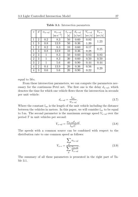
3.3 Light Controlled Intersection Model 27Table 3.1: Intersection parameterss d α s→d w s→d t s→d d s→d V s→d V s→[m·s −1 ] [s] [s/uv] [uv/s] [uv/s]1 2 0.2 8.3 50 0.60 0.831 3 0.8 13.9 50 0.36 1.391.231 2 0.2 8.3 10 0.60 0.171 3 0.8 13.9 10 0.36 0.280.252 3 1 8.3 50 0.60 0.83 0.832 3 1 8.3 30 0.60 0.50 0.503 2 1 5.6 40 0.90 0.44 0.444 2 0.4 13.9 20 0.36 0.564 3 0.6 5.6 20 0.90 0.220.29equal to 50 s.From these intersection parameters, we can compute the parameters necessaryfor the continuous Petri net. The first one is the delay d s→d , whichdenotes the time for which one vehicle flows throw the intersection in secondsper unit vehicle:d s→d =l uv. (3.7)w s→dWhere the constant l uv is the length of the unit vehicle including the distancebetween the vehicles in meters. In this paper, we will consider l uv to be equalto 5 m. The second parameter is the maximum average speed V s→d over theperiod T in unit vehicles per second:V s→d = w s→dt s→dl uv C . (3.8)The speeds with a common source can be combined with respect to thedistribution rate to one common speed as follows:∑ddα s→dV s→ = ∑ α s→d. (3.9)V s→dThe summary of all these parameters is presented in the right part of Table3.1.