Cowell's Method for Heliocentric Orbits - Orbital and Celestial ...

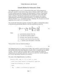
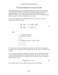
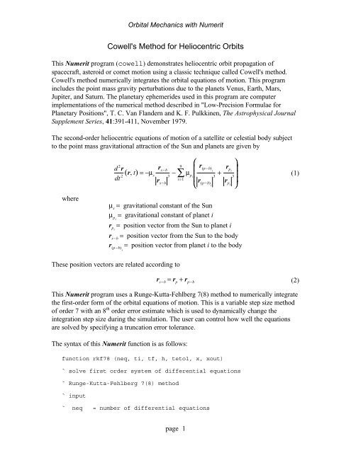
Orbital Mechanics with NumeritCowell's Method for Heliocentric OrbitsThis Numerit program (cowell) demonstrates heliocentric orbit propagation ofspacecraft, asteroid or comet motion using a classic technique called Cowell's method.Cowell's method numerically integrates the orbital equations of motion. This programincludes the point mass gravity perturbations due to the planets Venus, Earth, Mars,Jupiter, and Saturn. The planetary ephemerides used in this program are computerimplementations of the numerical method described in "Low-Precision Formulae forPlanetary Positions", T. C. Van Flandern and K. F. Pulkkinen, The Astrophysical JournalSupplement Series, 41:391-411, November 1979.The second-order heliocentric equations of motion of a satellite or celestial body subjectto the point mass gravitational attraction of the Sun and planets are given byd 2 rdt 2 (r, t) = −µ sr s−b∑r s−b3 − 9i=1µ pi⎛⎜⎜⎜⎝r (p−b)i+ r p i3 3r (p−b)ir pi⎞⎟⎟⎟⎠(1)whereµ s= gravitational constant of the Sunµ pi= gravitational constant of planet ir pi= position vector from the Sun to planet ir s−b= position vector from the Sun to the bodyr (p−b)i= position vector from planet i to the bodyThese position vectors are related according tor s−b= r p+ r p−b(2)This Numerit program uses a Runge-Kutta-Fehlberg 7(8) method to numerically integratethe first-order form of the orbital equations of motion. This is a variable step size methodof order 7 with an 8 th order error estimate which is used to dynamically change theintegration step size during the simulation. The user can control how well the equationsare solved by specifying a truncation error tolerance.The syntax of this Numerit function is as follows:function rkf78 (neq, ti, tf, h, tetol, x, xout)` solve first order system of differential equations` Runge-Kutta-Fehlberg 7(8) method` input` neq= number of differential equationspage 1

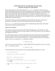
Orbital Mechanics with Numerit` ti = initial simulation time` tf = final simulation time` h = initial guess for integration step size` tetol = truncation error tolerance (non-dimensional)` x = integration vector at time = ti` output` xout = integration vector at time = tfThis algorithm requires the following statement the first time it is called.rkcoef = 1This statement is placed in the main program and is used to initialize the integrationcoefficients for this numerical method. The value of rkcoef is passed to the rkf78function using a common rkcoef statement in the main program. The rkf78 functionwill then set this to 0 after the coefficients are calculated.This function also requires a second function which defines the user's system of first-orderdifferential equations. The format of this function is given byfunction orbeqm (time, y, ydot)` first order equations of orbital motion` cowell's method` input` time = simulation time (seconds)` y = state vector` output` ydot = integration vectorwhere orbeqm is the actual name of the user-coded function. The function parameter listshould be exactly as shown here. The main program uses "rerouting" to tell the rkf78function which equations of motion function to use. For this example the code isorbeqm -> ceqmThe cowell program will prompt you for the name of an orbital elements data file,including the file name extension. It will also prompt you for the initial calendar date anduniversal time. The final request asks for the simulation duration in days.The orbital elements data file contains true-of-date, heliocentric ecliptic classical orbitalelements. It is a simple ascii text file created with a text editor. The format and contents ofa typical data file are as follows:page 2

Orbital Mechanics with Numeritcalendar date of perihelion passage(1

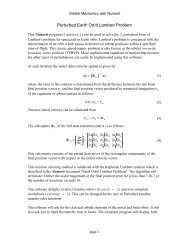
Orbital Mechanics with Numerit58.1306470436 107.680222659 219.493562547 27855.6991624perihelion radius = 0.58748972935 AUThe initial calendar date and universal time for this example were January 1, 1986 at 0hours UT. The simulation period was 120 days and the RKF truncation tolerance was1.0e-8. This tolerance is "hard-wired" in the code (tetol) and can be easily changedby the user. Smaller values of tetol will predict the orbit more accurately at the expenseof longer run times.page 4