The Circular Restricted Three-body Problem

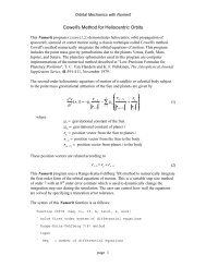
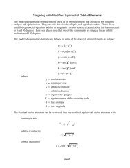
Celestial Computing with NumeritThe Circular Restricted Three-body ProblemThis Numerit program (g3body) graphically displays motion in the circular-restrictedthree-body problem (CRTBP). This algorithm and program examples are based on themethods described in "Periodic Orbits in the Restricted Three-Body Problem withEarth-Moon Masses", by R. A. Broucke, JPL TR 32-1168, 1968. In the discussion whichfollows, subscript 1 is the Earth and subscript 2 is the Moon.The system of second order vector differential equations of motion of a point masssatellite in the CRTBP are given byd 2 xdt − 2 dy2 dt − x = −(1 − µ) x−x 1− µ x−x 2r13 x23d 2 ydt − 2 dxy− y = −(1 − µ) − µ y 2 dt r13 x23(1)wherex = x component of positiony = y component of positionx 1= −µx 2= 1 − µµ = Earth-Moon mass ratio = m 1m 2≈ 1 81.27r 2 1 = (x − x 1) 2 + y 2r 2 2 = (x − x 2) 2 + y 2The motion of the spacecraft is displayed in a coordinate system which is rotating aboutthe center-of-mass or barycenter of the Earth-Moon system. The motion is confined to thex-y plane.For convenience, the problem is formulated in canonical units. The unit of length is takento be the constant distance between the Earth and Moon, and the unit of time is chosensuch that the Earth and Moon have an angular velocity ω about the barycenter equal to 1.Kepler's third law is thenω 2 m 1m 23= g(m1 + m 2) = 1(2)In his technical report, Professor Brouke calls these synodical coordinates.page 1

Celestial Computing with NumeritIn his prize memoir of 1772, Joseph-Louis Lagrange proved that there are fiveequilibrium points in the circular-restricted three-body problem. If we place a satellite orcelestial body at one of these points with zero initial velocity, it will stay therepermanently. These special positions are also called libration points.For the Earth-Moon mass ratio value of , the x and y coordinates of these five equilibriumpoints L iare as follows:L 1 x = +0.836892919 y = 0L 2 x = +1.155699520 y = 0L 3 x = -1.005064520 y = 0L 4 x = +0.487844901 y = +0.866025404L 5 x = +0.487844901 y = +0.866025404Three of these libration points are on the x-axis and the other two form equilateraltriangles with the positions of the Earth and Moon.The program begins by asking you to select from 4 main program options. The first threeoptions will display typical periodic orbits about the respective libration point. The initialconditions for each of these orbits are as follows:(1) periodic orbit about the L 1libration point(2) periodic orbit about the L 2libration point(3) periodic orbit about the L 3libration pointx 0= 0.300000161y· 0 = −2.536145497µ = 0.012155092t f= 5.349501906x 0= 2.840829343y· 0 = −2.747640074µ = 0.012155085t f= 11.933318588x 0= −1.600000312y· 0 = 2.066174572µ = 0.012155092t f= 6.303856312page 2

Celestial Computing with NumeritNotice that each orbit is defined by an initial x-component of position, x 0, an initialy-component of velocity, y· 0, a value of Earth-Moon mass ratio µ , and an orbital periodor final time t f. The initial y-component of position and x-component of velocity for eachthese orbits is equal to zero. The software will draw the location of the libration point onthe graphics display.If you would like to experiment with your own initial conditions, select option 4. Theprogram will then prompt you for the initial x and y components of the orbit's position andvelocity vector, and the value of to use in the simulation. The software will also ask for aninitial and final time to run the simulation, and an integration step size. The value 0.01 is agood number for step size.Here is a short list of initial conditions for several other periodic orbits which you maywant to display with this program.(1) Retrograde periodic orbit about m 1x 0= −2.499999883y· 0 = 2.100046263µ = 0.012155092t f= 11.99941766(2) Direct periodic orbit about m 1x 0= 0.952281734y· 0 = −0.957747254µ = 0.012155092t f= 6.450768946(3) Direct periodic orbit about m 1and m 2x 0= 3.147603117y· 0 = −3.07676285µ = 0.012155092t f= 12.567475674(4) Direct periodic orbit about m 2x 0= 1.399999991y· 0 = −0.9298385561µ = 0.012155092t f= 13.775148738page 3

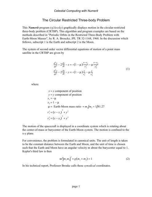
Celestial Computing with NumeritThe following is a plot of a periodic orbit about the L 2libration point. This plot wascreated by selecting program option 2.321y coordinate0-1-2-3-3 -2 -1 0 1 2 3x coordinateFigure 1. Periodic Orbit about the L 2 Libration PointFor a correct graphic display, the Width and Height dimensions should be the same as wellas the x and y axes scales. You can change these properties interactively by doubleclicking on this graph with the left mouse button.page 4