PDF Report - Orbital and Celestial Mechanics Website

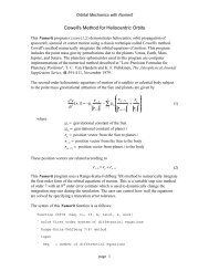
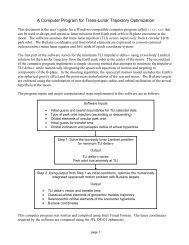
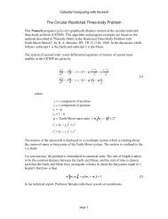
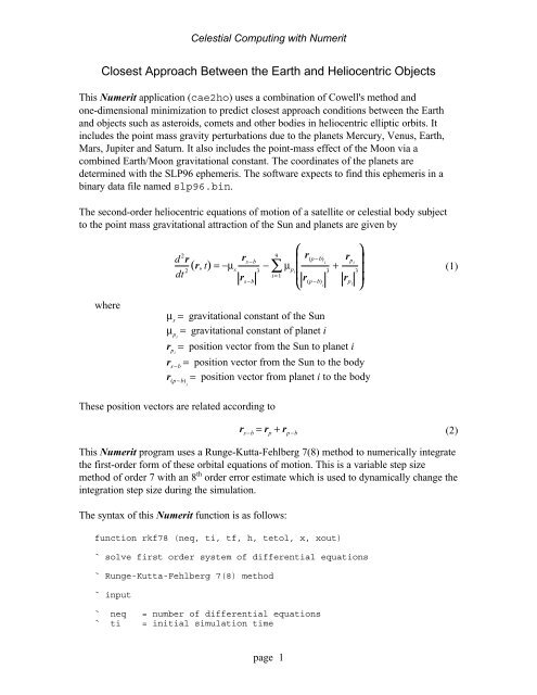
Celestial Computing with NumeritClosest Approach Between the Earth and Heliocentric ObjectsThis Numerit application (cae2ho) uses a combination of Cowell's method andone-dimensional minimization to predict closest approach conditions between the Earthand objects such as asteroids, comets and other bodies in heliocentric elliptic orbits. Itincludes the point mass gravity perturbations due to the planets Mercury, Venus, Earth,Mars, Jupiter and Saturn. It also includes the point-mass effect of the Moon via acombined Earth/Moon gravitational constant. The coordinates of the planets aredetermined with the SLP96 ephemeris. The software expects to find this ephemeris in abinary data file named slp96.bin.The second-order heliocentric equations of motion of a satellite or celestial body subjectto the point mass gravitational attraction of the Sun and planets are given byd 2 rdt 2 (r, t) = −µ sr s−b∑r s−b3 − 9i=1µ pi⎛⎜⎜⎜⎝r (p−b)i+ r p i3 3r (p−b)ir pi⎞⎟⎟⎟⎠(1)whereµ s= gravitational constant of the Sunµ pi= gravitational constant of planet ir pi= position vector from the Sun to planet ir s−b= position vector from the Sun to the bodyr (p−b)i= position vector from planet i to the bodyThese position vectors are related according tor s−b= r p+ r p−b(2)This Numerit program uses a Runge-Kutta-Fehlberg 7(8) method to numerically integratethe first-order form of these orbital equations of motion. This is a variable step sizemethod of order 7 with an 8 th order error estimate which is used to dynamically change theintegration step size during the simulation.The syntax of this Numerit function is as follows:function rkf78 (neq, ti, tf, h, tetol, x, xout)` solve first order system of differential equations` Runge-Kutta-Fehlberg 7(8) method` input` neq` ti= number of differential equations= initial simulation timepage 1

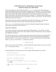
Celestial Computing with Numerit` tf = final simulation time` h = initial guess for integration step size` tetol = truncation error tolerance (non-dimensional)` x = integration vector at time = ti` output` xout = integration vector at time = tfThis function requires that the following statement be executed prior to the first timerkf78 is called.rkcoef = 1This statement is placed in the main program and is used to initialize the integrationcoefficients for this numerical method. The value of rkcoef is passed to the rkf78function using a common rkcoef statement in the main program. The rkf78 functionwill then set this "flag" to 0 after the coefficients are calculated.This function also requires a second function which defines the user's system of first-ordervector differential equations. The format of this function is given byfunction orbeqm (time, y, ydot)` first order equations of orbital motion` cowell's method` input` time = simulation time (seconds)` y = state vector` output` ydot = integration vectorwhere orbeqm is the actual name of the user-coded function. The function parameter listshould be exactly as shown here. The main program uses "rerouting" to tell the rkf78function which equations of motion function to use. For this example the code isorbeqm -> caeqmThis software also uses a one-dimensional optimization algorithm due to Richard Brent tosolve the close approach problem. Additional information about this numerical method canbe found in Algorithms for Minimization Without Derivatives, R.P. Brent, Prentice-Hall,1972. As the title of this book indicates, this algorithm does not require derivatives of theobjective function. This feature is important because the analytic first derivative of manyobjective functions is difficult to derive and code. The objective function for this classicalcelestial mechanics problem is the scalar geocentric distance of the heliocentric body.page 2

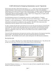
Celestial Computing with NumeritThe software will ask you for the name of a simple ASCII input file which defines thesimulation. When responding to this request be sure to include the file name extension.The software will also ask you for the total simulation (search) duration in days and anEarth-to-body close approach constraint in astronomical units. The software will ignoreany close approaches that are larger than the close approach constraint. Please note theproper units and coordinate system (J2000 equinox) of the input orbital elements. Noticealso that time on the Barycentric Dynamical Time (TDB) scale is used.The following is a typical input data file (xf11n.dat) for this program. It contains theJ2000 dynamical equator and equinox heliocentric orbital elements of the asteroid 1997XF 11. This file was created using data available on the Horizons ephemeris system whichis located on the Internet at http://ssd.jpl.nasa.gov/horizons.html. Additional informationabout NEOs (Near Earth Objects) can also be found at http://newton.dm.unipi.it/neodys/.Do not change the total number of lines or the order of annotation and data in this file.The software expects to find exactly 34 lines of information in the input data file. The lastdata item of this file defines the fundamental plane of the J2000 coordinate system.initial calendar date(1

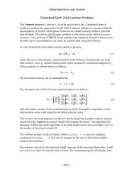
Celestial Computing with NumeritThe conversion of a position r and velocity vector v from the J2000 ecliptic frame(subscript ec) to the J2000 equatorial frame (subscript eq) is given by the followingmatrix-vector relationship:r⎡⎢⎢⎣1 0 0⎡⎢ ⎣ v⎤⎥= 0 cosε −sinε⎦ eq 0 sinε cosε⎤⎥⎥ ⎦⎡⎢⎣rv⎤⎥⎦ ec(3)In this expression ε is the J2000 obliquity of the ecliptic.The following is the draft output created by this program for this example. The programoutput and all internal calculations are performed in the J2000 dynamical equinox andequator coordinate system. All angular elements in this output are in degrees.initial heliocentric orbital elements(J2000 dynamical equinox and equator)October 20, 199800 h 00 m 00 ssemimajor axis (au) 1.441779254846407eccentricity 0.4836740409964595inclination 20.17287833484568argument of perihelion 322.8014264370198right ascension of ascending node 353.3298230482567true anomaly 221.6544086526512close approach conditionsOctober 31, 200200 h 30 m 40.5942 sheliocentric orbital elements(J2000 dynamical equinox and equator)semimajor axis (AU) 1.442267124200949eccentricity 0.4841223848226988inclination 20.16564547782856argument of perihelion 322.7924266589294right ascension of ascending node 353.3467738153024true anomaly 77.11093827535139geocentric distance (AU) 0.06355264422584024page 4