PDF document - Orbital and Celestial Mechanics Website

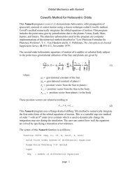
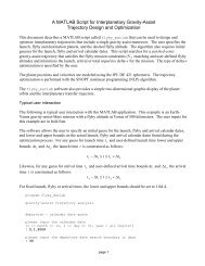
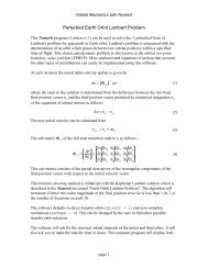
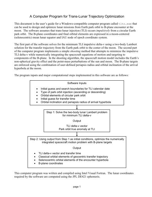
A Computer Program for Trans-Lunar Trajectory OptimizationThis document is the user’s guide for a Windows-compatible computer program called tlto.exe thatcan be used to design and optimize lunar missions from Earth park orbit to B-plane encounter at themoon. The software assumes that trans-lunar injection (TLI) occurs impulsively from a circular Earthpark orbit. The B-plane coordinates and final orbital elements are expressed in a moon-centered(selenocentric) mean lunar equator and IAU node of epoch coordinate system.The first part of the software solves for the minimum TLI impulsive delta-v using a two-body Lambertsolution for the transfer trajectory from the Earth park orbit to the center of the moon. The second partof the computer program implements a simple shooting method that attempts to minimize the impulsiveTLI delta-v while numerically integrating the spacecraft equations of motion and targeting tocomponents of the B-plane. In the shooting algorithm, the spacecraft motion model includes the Earth’snon-spherical gravity effect and the point-mass perturbations of the sun and moon. The B-plane targetsare enforced using the combination of user-defined periapsis radius and orbital inclination of the arrivalhyperbola at the moon.The program inputs and major computational steps implemented in this software are as follows:Software InputsInitial guess and search boundaries for TLI calendar dateType of park orbit injection (ascending or descending)Orbital elements of circular park orbitInitial guess for transfer timeOrbital inclination and periapsis radius of arrival hyperbolaStep 1: Solve the two-body lunar Lambert problemfor minimum TLI delta-vOutputTLI delta-v vectorPark orbit true anomaly at TLIStep 2: Using output from Step 1 as initial conditions, optimize the numericallyintegrated spacecraft motion problem with B-plane targetsOutputTLI delta-v vector and transfer timeClassical orbital elements of geocentric transfer trajectorySelenocentric orbital elements of the encounter hyperbolaB-plane coordinatesThis computer program was written and compiled using Intel Visual Fortran. The lunar coordinatesrequired by the software are computed using the JPL DE421 ephemeris.page 1

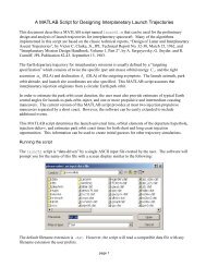
Program executionAn input file created by the user can be run from the command line or a simple batch file with astatement similar to the following:tlto tlto1.inIf the software is executed without an input file on the command line, the computer program will displaythe following information screen and file name prompt:************************************* program tlto ** ** trans-lunar trajectory ** optimization ** ** April 22, 2013 *************************************please input the name of the simulation definition fileAt this point the user should input the name of a valid input file, including the filename extension.To create a DOS command window in Windows 7, select start, then All Programs, then Accessoriesand finally Command Prompt. The size, font and other characteristics of the screen can be controlledby the user with the c:\ icon in the upper left corner of the window. To log into the subdirectory createdduring the installation of the Fortran executable and support files, type root:\ and then cd subdirectoryfrom the DOS command line where root is the name of the root directory, usually c:, and subdirectory isthe name of the subdirectory created by the user.The DOS command line prompt looks similar to C:\tlto>_.Input data file format and contentsThe tlto computer program is “data-driven” by a simple text file created by the user. This sectiondescribes a typical input data file. In the following discussion the actual input file contents are incourier font and all explanations are in times italic font. Each data item within an input file ispreceded by one or more lines of annotation text. Do not delete any of these annotation lines or increaseor decrease the number of lines reserved for each comment. However, you may change them to reflectyour own explanation. The annotation line also includes the correct units and when appropriate, thevalid range of the input.The first five lines of any input file are reserved for user comments. These lines are ignored by thesoftware. However the input file must begin with five and only five initial text lines.*************************************** input file for program tlto* tlto1.in – December 4, 2010* polar lunar orbit at 100 km altitude**************************************page 2

The software allows the user to specify an initial guess for the TLI calendar date and lower and upperbounds on the actual date found during both the two-body and numerically integrated TLI delta-voptimization processes. For any guess for the TLI time t TLIand user-defined lower and upper bounds t land t u, the actual TLI time t is constrained as follows:t t t t tTLI l TLI uThe first five inputs define the initial guesses for the TLI calendar date and the lower and upper bounds,respectively. Be sure to include all four digits of the calendar year. The first set of bounds is usedduring the two-body optimization, and the second set is used during the numerical integration and B-plane targeting.The TLI calendar date is a control variable in the NLP formulation and must always have a lower andupper bound. For a fixed TLI calendar date, input small values (e.g., plus and minus 1.0e-8) for thebounds.initial guess for TLI calendar date (month, day, year)9,15,2008lower bound for TLI calendar date search (two-body optimization; hours)0.0upper bound for TLI calendar date search (two-body optimization; hours)+24.0lower bound for TLI calendar date search (integrated optimization; hours)-12.0upper bound for TLI calendar date search (integrated optimization; hours)+12.0The next input is the user’s initial guess for the TLI-to-B-plane transfer time, in hours.initial guess for transfer time (hours)110.0The next two numbers define the fixed values for park orbit altitude and orbital inclination. The altitudeius measured with respect to a spherical Earth model.***********************************circular park orbit characteristics***********************************altitude (kilometers)185.32orbital inclination (degrees)28.5This next integer input defines the type of TLI maneuver to perform. The software uses this indicator tocompute the park orbit RAAN.type of TLI maneuver(1 = ascending, 2 = descending)2This next integer input defines the type of targeting algorithm to use.page 3

The next two inputs are algorithm control parameters. The first input is the truncation error tolerancefor the Runge-Kutta-Felhberg integrator and determines how well the equations of orbital motion aresolved. The second input is the root-finding tolerance and it determines how accurately close approachto the moon is predicted.****************************algorithm control parameters****************************truncation error tolerance1.0d-12root-finding tolerance1.0d-8The final two inputs specify the name of the solution disk file and the time step at which the data iscreated and written to this file.***************************output file characteristics***************************name of output data filetlto1.csvprint step size (minutes)10.0Program example and trajectory graphicsThe following is the solution created by the computer program for this example. The output isorganized by the following major sections:First pass1. optimized two body Lambert solution2. TLI delta-v vector and magnitude3. pre-TLI and post-TLI flight conditionsTargeting pass1. pre-TLI and post-TLI flight conditions2. TLI delta-v vector and magnitude3. time and conditions at lunar closest approach4. classical orbital elements of the lunar transfer trajectory5. B-plane coordinates at closest approach to the moonThe first output section summarizes the optimized two-body Lambert solution. The solution is presentedin the Earth mean equator of J2000 coordinate system (EME2000). The trajectory characteristics aregiven before and after the impulsive TLI maneuver. The event time is provided in both UniversalCoordinated Time (UTC) and Barycentric Dynamical Time (TDB).page 5

======================================two-body lunar trajectory optimization======================================input data file ==> tlto1.indescending transfertime and conditions prior to TLI(geocentric Earth mean equator and equinox J2000)-------------------------------------------------UTC calendar date September 15, 2008UTC time 13:29:13.655UTC Julian date 2454725.06196359TDB time 13:30:18.837TDB Julian date 2454725.06271802sma (km) eccentricity inclination (deg) argper (deg)0.656345630000D+04 0.111646925668D-15 0.285000000000D+02 0.000000000000D+00raan (deg) true anomaly (deg) arglat (deg) period (hrs)0.357108632971D+03 0.242927962813D+03 0.242927962813D+03 0.146996629514D+01rx (km) ry (km) rz (km) rmag (km)-.324237192596D+04 -.497888348087D+04 -.278867391059D+04 0.656345630000D+04vx (kps) vy (kps) vz (kps) vmag (kps)0.677307078339D+01 -.346292269424D+01 -.169231904268D+01 0.779296254099D+01time and conditions after TLI(geocentric Earth mean equator and equinox J2000)-------------------------------------------------UTC calendar date September 15, 2008UTC time 13:29:13.655UTC Julian date 2454725.06196359TDB time 13:30:18.837TDB Julian date 2454725.06271802sma (km) eccentricity inclination (deg) argper (deg)0.187780715202D+06 0.965047229195D+00 0.285000000000D+02 0.242927927168D+03raan (deg) true anomaly (deg) arglat (deg) period (hrs)0.357108632971D+03 0.356447377822D-04 0.242927962813D+03 0.224949464232D+03rx (km) ry (km) rz (km) rmag (km)-.324237192596D+04 -.497888348087D+04 -.278867391059D+04 0.656345630000D+04vx (kps) vy (kps) vz (kps) vmag (kps)0.949449861264D+01 -.485433249196D+01 -.237229666009D+01 0.109241859784D+02trans-lunar injection delta-v vector and magnitude(geocentric Earth mean equator and equinox J2000)-------------------------------------------------page 6

deltav-x 2721.42782925067 meters/seconddeltav-y -1391.40979772003 meters/seconddeltav-z -679.977617407291 meters/seconddeltav 3131.22343744202 meters/secondeci unit thrust vector0.869126040865955 -0.444366180031124 -0.217160362712021rtn unit thrust vector1.065917010975581E-006 0.9999999999994322.081668171172169E-015The components of the unit thrust vector of the TLI impulsive maneuver are displayed in both the Earthcentered-inertial(ECI) and radial, tangential and normal (RTN) coordinate systems.This section of the program output is created after the B-plane targeting problem has been solved. Itincludes a summary of the solution, the TLI delta-v vector and magnitude, the final B-plane coordinatesand the orbital elements and state vector of the incoming hyperbola.=======================optimal n-body solution=======================descending transfertransfer time 106.519756112248 hourstrans-lunar injection delta-v vector and magnitude(geocentric Earth mean equator and equinox J2000)-------------------------------------------------deltav-x 2685.47702093217 meters/seconddeltav-y -1485.54512251347 meters/seconddeltav-z -629.489861744947 meters/seconddeltav 3132.87226471460 meters/secondeci unit thrust vector0.857193269951853 -0.474179920849342 -0.200930586553070rtn unit thrust vector3.929610390119714E-004 0.999999922789293-1.740973091191034E-006time and conditions prior to TLI(geocentric Earth mean equator and equinox J2000)-------------------------------------------------UTC calendar date September 15, 2008UTC time 09:54:55.649UTC Julian date 2454724.91314409TDB time 09:56:00.832TDB Julian date 2454724.91389851page 7

sma (km) eccentricity inclination (deg) argper (deg)0.656345630000D+04 0.716042246482D-16 0.285000000000D+02 0.000000000000D+00raan (deg) true anomaly (deg) arglat (deg) period (hrs)0.353245173740D+03 0.245118791050D+03 0.245118791050D+03 0.146996629514D+01rx (km) ry (km) rz (km) rmag (km)-.335780398217D+04 -.487156385281D+04 -.284112242738D+04 0.656345630000D+04vx (kps) vy (kps) vz (kps) vmag (kps)0.668164145782D+01 -.369300013531D+01 -.156450714128D+01 0.779296254099D+01time and conditions after TLI(geocentric Earth mean equator and equinox J2000)-------------------------------------------------UTC calendar date September 15, 2008UTC time 09:54:55.649UTC Julian date 2454724.91314409TDB time 09:56:00.832TDB Julian date 2454724.91389851sma (km) eccentricity inclination (deg) argper (deg)0.191022462974D+06 0.965640395831D+00 0.285000120341D+02 0.245105601643D+03raan (deg) true anomaly (deg) arglat (deg) period (hrs)0.353245228119D+03 0.131416178811D-01 0.245118743261D+03 0.230799647130D+03rx (km) ry (km) rz (km) rmag (km)-.335780398217D+04 -.487156385281D+04 -.284112242738D+04 0.656345630000D+04vx (kps) vy (kps) vz (kps) vmag (kps)0.936711847875D+01 -.517854525782D+01 -.219399700303D+01 0.109258346332D+02time and conditions at lunar closest approach(geocentric Earth mean equator and equinox of J2000)----------------------------------------------------UTC calendar date September 19, 2008UTC time 20:26:06.771UTC Julian date 2454729.35146726TDB time 20:27:11.954TDB Julian date 2454729.35222168sma (km) eccentricity inclination (deg) argper (deg)-.226037830064D+06 0.262793126648D+01 0.901673932456D+02 0.161060207106D+03raan (deg) true anomaly (deg) arglat (deg)0.231778348616D+03 0.354652795765D+03 0.155713002871D+03rx (km) ry (km) rz (km) rmag (km)0.207825892551D+06 0.264611286018D+06 0.151828443552D+06 0.369137658028D+06vx (kps) vy (kps) vz (kps) vmag (kps)0.431679155458D+00 0.539374509368D+00 -.185628181220D+01 0.198067006867D+01page 8

time and conditions at lunar closest approach(selenocentric lunar mean equator & IAU node of epoch)------------------------------------------------------UTC calendar date September 19, 2008UTC time 20:26:06.771UTC Julian date 2454729.35146726TDB time 20:27:11.954TDB Julian date 2454729.35222168sma (km) eccentricity inclination (deg) argper (deg)-.683169467107D+04 0.126904013040D+01 0.899999999599D+02 0.140405474608D+03raan (deg) true anomaly (deg) arglat (deg)0.146641367110D+03 0.360000000000D+03 0.140405474608D+03rx (km) ry (km) rz (km) rmag (km)0.118297039598D+04 -.778800401735D+03 0.117144998570D+04 0.183800002517D+04vx (kps) vy (kps) vz (kps) vmag (kps)0.130967217408D+01 -.862213640865D+00 -.189576658616D+01 0.246020009659D+01b-plane coordinates of incoming hyperbola(selenocentric lunar mean equator & IAU node of epoch)------------------------------------------------------b-magnitude 5337.74803144691 kilometersb dot r -5337.74803144691 kilometersb dot t3.733693318963560E-006 kilometerstheta 270.000000040078 degreesv-infinity 847.145240428195 meters/secondr-periapsis 1838.00002516655 kilometersdecl-asy 1.59325896718781 degreesrasc-asy 326.641367108400 degreesselenocentric flight path angle -1.078655371150484E-011 degrees----------------------------------------------------coordinates of the moon at closest approach(geocentric Earth mean equator and equinox of J2000)----------------------------------------------------UTC calendar date September 19, 2008UTC time 20:26:06.771UTC Julian date 2454729.35146726TDB time 20:27:11.954TDB Julian date 2454729.35222168sma (km) eccentricity inclination (deg) argper (deg)0.387057904331D+06 0.469260710975D-01 0.274682409204D+02 0.654909165021D+02raan (deg) true anomaly (deg) arglat (deg) period (hrs)0.352456394178D+03 0.357084293759D+03 0.625752102615D+02 0.665690548982D+03rx (km) ry (km) rz (km) rmag (km)0.206588660958D+06 0.265719415783D+06 0.151041328247D+06 0.368916204034D+06page 9

Z coordinate (ER)vx (kps) vy (kps) vz (kps) vmag (kps)-.880138031538D+00 0.553045427398D+00 0.224951785729D+00 0.106353444008D+01declination 24.1683467556695 degreesright ascension 52.1360342116955 degreesThe tlto software suite also includes an interactive MATLAB script called lplot.m that can be usedto create three-dimensional geocentric and selenocentric graphics of the solution. The graphics data isdisplayed at the user-defined step size provided in the input file. A plot step size of ten minutes isrecommended. However, for zoomed plots of either the geocentric or selenocentric trajectory, smallerplot step sizes will create “smoother” trajectory displays.Important note!!You must delete the first or “header” line of the tlto solution file in order for the lplot script to work.This script uses the MATLAB csvread function to read the data file which can only contain commaseparated-variable(CSV) numerical data. The lplot script will also create color Postscript graphicdisk files with a TIFF preview using MATLAB statements similar toprint -depsc -tiff -r300 tlto1.epsThe following is a plot of the geocentric transfer trajectory for this example. Please note that thecoordinates are displayed in the units of Earth radii (ER). The asterisk symbol is the position of themoon at the moment of trans-lunar injection and the park orbit trace is red. The interactive graphicfeatures of MATLAB will allow the user to rotate and “zoom” the displays in and out. Thesecapabilities allow the user to interactively find the “best” viewpoint as well as verify the basic orbitalgeometry of the geocentric and selenocentric trajectories.Geocentric Transfer Trajectory50403020100-10-20-300102030Y coordinate (ER)400-20-40-60X coordinate (ER)page 10

This next plot is a “zoomed” display of the first plot closer to the Earth. The initial park orbit isdisplayed in red, the transfer trajectory is blue, and an inertial, Earth-centered coordinate system is onthe plot. The x-axis of this system is red, the y-axis green and the z-axis blue. The location on the parkorbit at which TLI occurs is marked with a small dot symbol.0This plot illustrates the geocentric trajectory of the spacecraft in the vicinity of the moon. In thisdisplay, the location of the spacecraft when it enters the sphere-of-influence of the moon is marked witha blue asterisk. The spacecraft trajectory at closest approach to the moon is the small blue dot and thelocation of the moon at closest approach is the green asterisk.-10page 11

Z coordinate (MR)The following is a plot of the selenocentric hyperbola within the moon’s sphere-of-influence. Thecoordinate units are lunar radii (LR). The entry into the SOI is marked with an asterisk. In thisMATLAB script the radius of the moon’s SOI is “hardwired” to a value of 64,000 kilometers.Selenocentric Trajectory151050-5-10-15-2020 -3010-200-10-10-20 0Y coordinate (MR)X coordinate (MR)The final plot is a “zoomed” display of the previous plot. This display is labeled with a selenocentric,inertial coordinate system. The x-axis is red, the y-axis green and the z-axis blue. The small red dot isperiapsis of the approach hyperbola.page 12

Verification of the solutionAfter the n-body optimization finishes, the software will verify the solution by numerically integratingthe equations of motion using a Runge-Kutta-Fehlberg 7(8) numerical method. The integration startswith the position and velocity vector of the trans-lunar transfer orbit immediately after the TLIimpulsive maneuver and propagates to closest approach to the moon predicted by the software.The following is the verification summary for this example.===================================verification of the n-body solution===================================time and conditions at lunar closest approach(geocentric Earth mean equator and equinox of J2000)----------------------------------------------------UTC calendar date September 19, 2008UTC time 20:26:06.771UTC Julian date 2454729.35146726TDB time 20:27:11.954TDB Julian date 2454729.35222168sma (km) eccentricity inclination (deg) argper (deg)-.226037824690D+06 0.262793130505D+01 0.901673927406D+02 0.161060207167D+03raan (deg) true anomaly (deg) arglat (deg)0.231778348844D+03 0.354652795710D+03 0.155713002877D+03rx (km) ry (km) rz (km) rmag (km)0.207825892558D+06 0.264611286027D+06 0.151828443521D+06 0.369137658025D+06vx (kps) vy (kps) vz (kps) vmag (kps)0.431679141547D+00 0.539374522535D+00 -.185628182291D+01 0.198067007926D+01time and conditions at lunar closest approach(selenocentric lunar mean equator & IAU node of epoch)------------------------------------------------------UTC calendar date September 19, 2008UTC time 20:26:06.771UTC Julian date 2454729.35146726TDB time 20:27:11.954TDB Julian date 2454729.35222168sma (km) eccentricity inclination (deg) argper (deg)-.683169495857D+04 0.126904011717D+01 0.899999999777D+02 0.140405474793D+03raan (deg) true anomaly (deg) arglat (deg)0.146641367130D+03 0.736558247354D-06 0.140405475530D+03rx (km) ry (km) rz (km) rmag (km)0.118297040379D+04 -.778800405836D+03 0.117144995460D+04 0.183800001211D+04page 13

vx (kps) vy (kps) vz (kps) vmag (kps)0.130967216081D+01 -.862213632161D+00 -.189576660132D+01 0.246020009815D+01b-plane coordinates of incoming hyperbola(selenocentric lunar mean equator & IAU node of epoch)------------------------------------------------------b-magnitude 5337.74810923454 kilometersb dot r -5337.74810923454 kilometersb dot t2.076305861464789E-006 kilometerstheta 270.000000022287 degreesv-infinity 847.145222603009 meters/secondr-periapsis 1838.00001210839 kilometersdecl-asy 1.59325954678117 degreesrasc-asy 326.641367129470 degreesselenocentric flight path angle4.119460026174752E-007 degreesTechnical discussionThis section provides additional details about the numerical algorithms used in this computer program.The computational methods discussed here include solving the two body Lambert problem, the methodused for propagating the spacecraft’s geocentric trajectory, the algorithm used for targeting to the B-plane, and the geocentric-to-selenocentric coordinate transformation.Nonlinear programming problemA trajectory optimization problem can be described by a system of dynamic variablesyz uconsisting of the state variables y and the control variables u for any time t. In this discussion vectorsare denoted in bold.The system dynamics are defined by a vector system of ordinary differential equations called the stateequations that can be represented as follows:tt d yy t, t, , tdt f y u p where p is a vector of problem parameters that is not time dependent.The initial dynamic variables at time 0conditions at the final timefboundary values of the trajectory problem.ψ 0 ψ y t0 , u t0 , t0and the terminalt are defined by t are defined by ψf ψ tf, tf, t y uf . These conditions are called theg y t , u t , t0 .The problem may also be subject to path constraints of the form page 14

For any mission time t there are also simple bounds on the state variablesthe control variableslty y yultu u uuand the problem parametersltp p pThe basic nonlinear programming problem (NLP is to determine the control vector history and problemparameters that minimize the scalar performance index or objective function given byu 0 0 f J t , t , t , tf,y y p while satisfying all the user-defined mission constraints.During the two-body trajectory optimization, the control variables are the TLI calendar date and the trueanomaly of the TLI maneuver. For the numerical integration optimization, the control variables consistof the TLI calendar date, the RAAN of the park orbit, the true anomaly of the TLI maneuver, and theCartesian components of the TLI delta-v vector.For both types of optimization, the objective function or performance index is the scalar magnitude ofthe TLI impulsive delta-v.In addition to the bounds on the TLI calendar date mentioned earlier, the true anomaly during the twobodyoptimization is bounded according to180 180During the second part of the trajectory optimization, the RAAN and true anomaly bounds are 30 30TBTB 30 30TBwhere TBand TBare the RAAN and true anomaly found during the two-body optimization. Thebounds on the components of the TLI delta-v are given by v 0.1 v vx, y,z v 0.1 v where v is the scalar magnitude of the two-body TLI delta-v vector.The final boundary conditions are the B-plane coordinates of the incoming selenocentric hyperbola.TBpage 15

Solving the two body Lambert problemLambert’s problem is concerned with the determination of an orbit that passes between two positionswithin a specified time-of-flight. This classic astrodynamic problem is also known as the orbital twopointboundary value problem (TPBVP).The time to traverse a trajectory depends only upon the length of the semimajor axis a of the transfertrajectory, the sum r i r fof the distances of the initial and final positions relative to a central body, andthe length c of the chord joining these two positions. This relationship can be stated as follows:From the following form of Kepler’s equationtof tof r r , c,aifwe can write3at t0 E esinE3at E E esinE sin E 0 0where E is the eccentric anomaly associated with radius r, E0is the eccentric anomaly at r 0, and t 0when r r0.At this point we need to introduce the following trigonometric sun and difference identities: a sinsin 2sin cos2 2 a cos cos 2sin sin2 2 a coscos 2cos cos2 2If we let E and E0 and substitute the first trig identity into the second equation above, we havethe following equation:With the two substitutions given by3a E E0 E E0t E E0 2sin ecos 2 2page 16

EE0 ecos cos2 2EE0 sin sin2 2the time equation becomesFrom the elliptic relationships given by3a t 2sin cos 2 2 r a 1ecosEx a cos E ey a sin E 1e2and some more manipulation, we have the following equations: r r c r r c s 2a 2a 2a a0 0cos1 1 1 r r c r r c s c 2a 2a 2a a0 0sin 1 1 1This part of the derivation makes use of the following three relationships: rrcos cos 12 2 202E E0 E E0 e sin sin sin 1 cos2 2 2 22 2 2 2x x0 y y0c sinsin 2 2 2a 2a 2aWith the use of the half angle formulas given bysins sins c2 2a2 2aand several additional substitutions, we have the time-of-flight form of Lambert’s theorempage 17

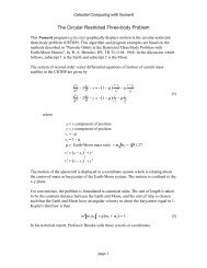
3at sin sin A discussion about the angles and can be found in “Geometrical Interpretation of the Angles and in Lambert’s Problem” by J. E. Prussing, AIAA Journal of Guidance and Control, Volume 2,Number 5, Sept.-Oct. 1979, pages 442-443.The algorithm used in this computer program is based on the method described in “A Procedure for theSolution of Lambert’s Orbital Boundary-Value Problem” by R. H. Gooding, Celestial Mechanics andDynamical Astronomy 48: 145-165, 1990. This iterative solution is valid for elliptic, parabolic andhyperbolic transfer orbits which may be either posigrade or retrograde, and involve one or morerevolutions about the central body.Modeling the spacecraft’s trajectoryThe spacecraft’s orbital motion is modeled with respect to the Earth mean equator and equinox of J2000(EME2000) coordinate system. The following figure illustrates the geometry of the EME2000coordinate system. The origin of this Earth-centered-inertial (ECI) inertial coordinate system is thegeocenter and the fundamental plane is the Earth’s mean equator. The z-axis of this system is normal tothe Earth’s mean equator at epoch J2000, the x-axis is parallel to the vernal equinox of the Earth’s meanorbit at epoch J2000, and the y-axis completes the right-handed coordinate system. The epoch J2000 isthe Julian Date 2451545.0 which corresponds to January 1, 2000, 12 hours Terrestrial Time (TT).This part of the trajectory analysis implements a special perturbation technique which numericallyintegrates the vector system of second-order, nonlinear differential equations of motion of a spacecraftgiven bya r, v, t r r, r, t a r a r, t a r,t g m spage 18

N n n R r n2 r m0 m m m ncos nsin n sinm S m C m PwhereSmnR r radius of the Earthgeocentric distance of the spacecraftm, C harmonic coefficientsn geocentric latitude of the spacecraft sin longitude of the spacecraft 1 right ascension of the spacecraft tan y x right ascension of Greenwichgg1zrRight ascension is measure positive east of the vernal equinox, longitude is measured positive east ofGreenwich, and latitude is positive above the Earth’s equator and negative below.For m 0, the coefficients are called zonal terms, when m n the coefficients are sectorial terms, andfor n m 0 the coefficients are called tesseral terms.The Legendre polynomials with argument sin are computed using recursion relationships given by:1P n P n Pn sin 2 1sin sin 1 sin0 0 0n n1 n2n1 nP sin 2n 1 cos P sin , m 0, m nnn11 P sin P sin 2n 1 cos P sin , m 0, m nm m mn n2 n1where the first few associated Legendre functions are given byjand P 0 for j i .i P sin 1, P sin sin , P sin cos0 0 10 1 1The trigonometric arguments are determined from expansions given byPoint-mass gravity of the sun and moon sin m 2cos sin m 1 sin m 2 cos m 2cos cos m 1 cos m 2 mtan m1 tan tanThe acceleration contribution of the moon represented by a point mass is given bypage 20

where rmmbremam r rmb emr, t m3 3mbrremgravitational constant of the moonposition vector from the moon to the satelliteposition vector from the Earth to the moonThe acceleration contribution of the sun represented by a point masses is given byas r rsb esr, t s3 3sbrreswhere rssbresgravitational constant of the sunposition vector from the sun to the satelliteposition vector from the Earth to the sunTo avoid numerical problems, use is made of Richard Battin’sf q function given bywheref qkq2 33qkqk qk 3 11qk kT 2 r r sTsskkkThe point-mass acceleration due to n gravitational bodies can now be expressed asnr f qkkdr s In these equations, skis the vector from the primary body to the secondary body,constant of the secondary body andk kto the primary body. The derivation of thek1k3kkis the gravitationald r s , where r is the position vector of the spacecraft relativef q functions is described in Section 8.4 of “AnIntroduction to the Mathematics and Methods of Astrodynamics, Revised Edition”, by Richard H.Battin, AIAA Education Series, 1999.In this computer program the heliocentric coordinates of the sun and moon are based on the JPLDevelopment Ephemeris DE421. These coordinates are provided in the Earth mean equator andequinox of J2000 coordinate system (EME2000). The name of this binary date file is de421.bin, andit must reside in the same directory as the tlto.exe computer program.page 21

Park orbit RAANFor a given TLI injection time, there are two possible locations on the initial park orbit at which toperform the propulsive maneuver. One opportunity occurs during the ascending part of the park orbitand the other during the descending motion. The park orbit RAAN at these two locations can bedetermined from spherical trigonometry relationships involving the park orbit inclination and the rightascension and declination of the moon at encounter.1ascending p 180 m sin tanm tan ip1descending p m sin tanm tanippwheremmi pright ascension of the moon at encounterdeclination of the moon at encounterpark orbit inclinationThese opportunities are valid whenever m ip.B-plane targetingThe derivation of B-plane coordinates is described in the classic JPL reports, “A Method of DescribingMiss Distances for Lunar and Interplanetary Trajectories” and “Some Orbital Elements Useful in SpaceTrajectory Calculations”, both by William Kizner. The following diagram illustrates the fundamentalgeometry of the B-plane coordinate system.page 22

The software solves the B-plane targeting problem by minimizing the delta-v vector at the TLI whilesatisfying two nonlinear equality constraint equations. These constraint equations are the differencesbetween components of the required B-plane and the B-plane components predicted by the software.Given the user-defined closest approach radius r caand orbital inclination i, and the incoming v-infinitymagnitude v and the right ascension and declination of the incoming asymptote vector at themoment of closest approach, the following series of equations can be used to determine the required B-plane target components:BTb costwhereBRb sin2r2b r r 1ca 2t 2 ca ca2vrcavtandcosi cos2 1cos sin 1 cos tan sin ,cos2 2sin sˆ z ˆ sx syz ˆ 0 0 1 TThe arrival asymptote unit vector Ŝ is given by coscosˆ S cossin sin where and are the declination and right ascension of the asymptote of the incoming hyperbola.Important note!!This technique only works for lunar orbit inclinations that satisfyi If this inequality is not satisfied, the software will print the following error messageb-plane targeting error!!|inclination| must be > |asymptote declination|page 23

It will also display the actual declination of the asymptote and stop. The user should then edit the inputfile, include a valid orbital inclination and restart the simulation.The following computational steps summarize the calculation of the predicted B-plane vector from amoon-centered position vector r and velocity vector v at closest approach.angular momentum vector h r vradius ratesemiparameterr r v r2ph rsemimajor axis a 2rv 2 orbital eccentricity e 1p atrue anomalyprcos sinerrhe1 tan sin ,cosB-plane magnitude B p afundamental vectorsr rz ˆ v r pˆ cosrˆsinz ˆ qˆ sinrˆcoszˆhS vectorB vectorT vectora bS pˆ q ˆ2 2 2 2a b a b2b abB pˆ q ˆ2 2 2 2a b a bT 2 2y x2 2x yS , S,0 TS SR vector R S T SzTy, SzTx,SxTy SyTxTargeting to the Selenocentric Periapsis Radius and Orbital InclinationFor this targeting option, the equality constraints enforced by the nonlinear programming algorithm areTpage 24

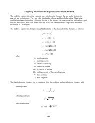
prca0cosihˆ0where rpand i are the user-defined periapsis radius and selenocentric orbital inclination, respectively.In the second equation h ˆzis the z-component of the spacecraft’s unit angular momentum vector atclosest approach to the moon.For both types of targeting techniques, closest approach is determined during the numerical integrationof the spacecraft equations of motion by finding the time since TLI at which the selenocentric flight pathangle is zero. This mission constraint is computed as follows rvsin0 rvwhere r and v are the spacecraft’s moon-centered position and velocity vectors, respectively.Geocentric-to-selenocentric coordinate transformationThis section describes the transformation of coordinates between the Earth mean equator and equinox2000 (EME2000) and lunar mean equator and IAU node of epoch coordinate systems. Thistransformation is used to compute the B-plane coordinates at encounter.The following diagram illustrates the orientation of the lunar mean equator and IAU node of epochcoordinate frame.zpage 25

A unit vector in the direction of the pole of the moon can be determined fromcospcospp ˆMoon sinp cosp sinp where pand pare the right ascension and declination of the lunar pole.The right ascension and declination of the lunar pole in the EME2000 coordinate system are given bythe following expressionsP 269.9949 0.0031T 3.8787sin E10.1204sin E20.0700sin E3 0.0172sin E4 0.0072sin E60.0052sin E10 0.0043sin E13P 66.5392 0.0130T 1.5419cos E10.0239cos E20.0278cos E3 0.0068cos E4 0.0029cos E60.0009cos E7 0.0008cos E10 0.0009cos E13where T is the time in Julian centuries given by T JDBarycentric Time (TDB) Julian Date.The trigonometric arguments, in degrees, for these equations are 2451545.0 / 36525 and JD is the DynamicalE1 125.045 0.0529921dE2 250.089 0.1059842dE3 260.008 13.0120009dE4 176.625 13.3407154dE6 311.589 26.4057084dE7 134.963 13.0649930dE10 15.134 0.1589763dE13 25.053 12.9590088dwhere d JD 2451545 is the number of days since January 1.5, 2000. These equations are given in“Report of the IAU Working Group on Cartographic Coordinates and Rotational Elements: 2009”,Celestial Mechanics and Dynamical Astronomy, 109: 101-135, 2011.The unit vector in the x-axis direction of this selenocentric coordinate system is given bywhere z xˆ zˆpˆMoonˆ 0 0 1 T. The unit vector in the y-axis direction can be determined usingpage 26

yˆpˆxˆFinally, the components of the matrix that transforms coordinates from the EME2000 system to themoon-centered (selenocentric) mean equator and IAU node of epoch system are as follows:Time systemsMoonM xˆyˆp ˆThis section is a brief explanation of the time scales used in this computer program.Coordinated Universal Time, UTCCoordinated Universal Time (UTC) is the time scale available from broadcast time signals. It is acompromise between the highly stable atomic time and the irregular earth rotation. UTC is theinternational basis of civil and scientific time.Terrestrial Time, TTTerrestrial Time is the time scale that would be kept by an ideal clock on the geoid - approximately, sealevel on the surface of the Earth. Since its unit of time is the SI (atomic) second, TT is independent ofthe variable rotation of the Earth. TT is meant to be a smooth and continuous “coordinate” time scaleindependent of Earth rotation. In practice TT is derived from International Atomic Time (TAI), a timescale kept by real clocks on the Earth's surface, by the relation TT = TAI + 32 s .184. It is the time scalenow used for the precise calculation of future astronomical events observable from Earth.TT = TAI + 32.184 secondsMoonTT = UTC + (number of leap seconds) + 32.184 secondsBarycentric Dynamical Time, TDBBarycentric Dynamical Time is the time scale that would be kept by an ideal clock, free of gravitationalfields, co-moving with the solar system barycenter. It is always within 2 milliseconds of TT, thedifference caused by relativistic effects. TDB is the time scale now used for investigations of thedynamics of solar system bodies.TDB = TT + periodic correctionswhere typical periodic corrections (USNO Circular 179) areTpage 27

TDB TT 0.001657sin 628.3076T 6.24010.000022sin 575.3385T4.29700.000014sin 1256.6152T6.19690.000005sin 606.9777T4.02120.000005sin 52.9691T0.44440.000002sin 21.3299T5.54310.000010Tsin 628.3076T4.2490 In this equation, the coefficients are in seconds, the angular arguments are in radians, and T is thenumber of Julian centuries of TT from J2000; T = (Julian Date(TT) – 2451545.0) / 36525.page 28

Algorithm resources“Lunar Trajectories”, NASA TN D-866, August 1961.“Earth-Moon Trajectories”, JPL Technical Report No. 32-503, May 1, 1964.“Three-Dimensional Lunar Trajectories”, V. A. Egorov, Mechanics of Space Flight Series, IsraelProgram for Scientific Translations, Jerusalem 1969.“Circumlunar Trajectory Calculations”, MIT Instrumentation Laboratory Report R-353, April 1962.“Optimal Low Thrust Trajectories to the Moon”, John T. Betts and Sven O. Erb, SIAM Journal onApplied Dynamical Systems, Vol. 2, No. 2, pp. 144-170, 2003.“Integrated Algorithm for Lunar Transfer Trajectories Using a Pseudostate Technique”, R. V. Ramanan,AIAA Journal of Guidance, Control and Dynamics, Vol. 25, No. 5, September-October 2002, pp. 946-952.“Nonimpact Lunar Transfer Trajectories Using the Pseudostate Technique”, R. V. Ramanan and V.Adimurthy, AIAA Journal of Guidance, Control and Dynamics, Vol. 28, No. 2, March-April 2005, pp.217-225.“Injection Conditions for Lunar Trajectories”, R. Kolenkiewicz and W. Putney, NASA TM X-55390,November 1965.“Coplanar Three-Body Trans-Earth Lunar Trajectory Simulation Methodology”, H. Ikawa, AIAA 88-0381, AIAA 26 th Aerospace Sciences Meeting, Reno, Nevada, January 11-14, 1988.“Lunar Constants and Models Document”, JPL D-32296, September 23, 2005.page 29

APPENDIX AContents of the Simulation Summary and CSV FilesThis appendix is a brief summary of the information contained in the simulation summary screendisplays and the CSV data files produced by the tlto software.The simulation summary screen display contains the following information:transfer time = total time from the TLI maneuver to closest approach at the moonUTC time = simulation event time on the UTC time scaleTDB time = simulation event time on the TDB time scalesma (km) = semimajor axis in kilometerseccentricity = orbital eccentricity (non-dimensional)inclination (deg) = orbital inclination in degreesargper (deg) = argument of perigee in degreesraan (deg) = right ascension of the ascending node in degreestrue anomaly (deg) = true anomaly in degreesarglat (deg) = argument of latitude in degrees. The argument of latitude is the sum oftrue anomaly and argument of perigee.period (min) = orbital period in minutesrx (km) = x-component of the spacecraft’s position vector in kilometersry (km) = y-component of the spacecraft’s position vector in kilometersrz (km) = z-component of the spacecraft’s position vector in kilometersrmag (km) = scalar magnitude of the spacecraft’s position vector in kilometersvx (km/sec) = x-component of the spacecraft’s velocity vector in kilometers per secondvy (km/sec) = y-component of the spacecraft’s velocity vector in kilometers per secondvz (km/sec) = z-component of the spacecraft’s velocity vector in kilometers per secondvmag (km/sec) = scalar magnitude of the spacecraft’s velocity vector in kilometers perseconddelta-vx = x-component of the TLI impulsive velocity vector in meters/seconddelta-vy = y-component of the TLI impulsive velocity vector in meters/seconddelta-vz = z-component of the TLI impulsive velocity vector in meters/seconddelta-v = scalar magnitude of the TLI maneuver in meters/secondsb-magnitude = magnitude of the b-plane vectorb dot r = dot product of the b-vector and r-vectorb dot t = dot product of the b-vector and t-vectorpage 30

theta = orientation of the b-plane vectorv-infinity = magnitude of incoming v-infinity vectorr-periapsis = periapsis of incoming hyperboladecl-asy = declination of incoming v-infinity vectorrasc-asy = right ascension of incoming v-infinity vectorThe comma-separated-variable disk file contains the following information:time (sec) = simulation time since TLI maneuver in secondstime (min) = simulation time since TLI maneuver in minutestime (hr) = simulation time since TLI maneuver in hoursre2sc-x (km) = x-component of the spacecraft’s geocentric position vector in kilometersre2sc-y (km) = y-component of the spacecraft’s geocentric position vector in kilometersre2sc-z (km) = z-component of the spacecraft’s geocentric position vector in kilometersre2sc-mag (km) = the spacecraft’s geocentric radius in kilometersve2sc-y (km/sec) = y-component of the spacecraft’s geocentric velocity vector inkilometers per secondve2sc-z (km/sec) = z-component of the spacecraft’s geocentric position vector inkilometers per secondve2sc-mag (km/sec) = the spacecraft’s geocentric speed in kilometers per secondrm2sc-x (km) = x-component of the spacecraft’s selenocentric position vector inkilometersrm2sc-y (km) = y-component of the spacecraft’s selenocentric position vector inkilometersrm2sc-z (km) = z-component of the spacecraft’s selocentric position vector in kilometersrm2sc-mag (km) = the spacecraft’s selocentric radius in kilometersvm2sc-y (km/sec) = y-component of the spacecraft’s selocentric velocity vector inkilometers per secondvm2sc-y (km/sec) = y-component of the spacecraft’s selocentric velocity vector inkilometers per secondvm2sc-z (km/sec) = z-component of the spacecraft’s selocentric position vector inkilometers per secondvm2sc-mag (km/sec) = the spacecraft’s selocentric speed in kilometers per secondre2m-x (km) = x-component of the moon’s geocentric position vector in kilometersre2m-y (km) = y-component of the moon’s geocentric position vector in kilometersre2m-z (km) = z-component of the moon’s geocentric position vector in kilometersre2m-mag (km) = the moon’s geocentric radius in kilometerssma-geo (km) = geocentric semimajor axis of the spacecraft in kilometerspage 31

ecc-geo = geocentric orbital eccentricity of the spacecraft(non-dimensional)incl-geo (deg) = geocentric orbital inclination of the spacecraft in degreesargper-geo (deg) = geocentric argument of perigee of the spacecraft in degreesraan-geo (deg) = geocentric right ascension of the ascending node of the spacecraft indegreestanom-geo (deg) = geocentric true anomaly of the spacecraft in degreessma-sel (km) = selocentric semimajor axis of the spacecraft in kilometersecc-sel = selocentric orbital eccentricity of the spacecraft(non-dimensional)incl-sel (deg) = selocentric orbital inclination of the spacecraft in degreesargper-sel (deg) = selocentric argument of perigee of the spacecraft in degreesraan-sel (deg) = selocentric right ascension of the ascending node of the spacecraft indegreestanom-sel (deg) = selocentric true anomaly of the spacecraft in degreesThe geocentric coordinates of the spacecraft and the TLI delta-v components are with respect to theEarth mean equator and equinox of J2000 (EME2000) coordinate system. The selenocentric coordinatesare with respect to the mean lunar equator and IAU node of epoch coordinate system.page 32