PDF document - Orbital and Celestial Mechanics Website

Program leo2geo_ocsContinuous Low-Thrust LEO-to-GEO Trajectory OptimizationThis document is the user’s manual for a Fortran computer program called leo2geo_ocs that uses theSparse Optimization Suite distributed by Applied Mathematical Analysis to solve the continuous, singlemaneuver,finite-burn low Earth orbit (LEO) to geosynchronous Earth orbit (GEO) orbit transferoptimization problem. The software attempts to maximize the final spacecraft mass. Since thissimulation involves a single continuous propulsive maneuver, this is equivalent to minimizing thepropellant mass required for the orbital maneuver.The important features of this scientific simulation are as follows:single, continuous thrust transfer trajectoryconstant propulsive thrust magnitudemodified equinoctial equations of motionnear-circular initial and final orbitstwo types of initial guess algorithmsnumerical verification of the optimal control solutionThe Sparse Optimization Suite is a direct transcription method that can be used to solve a variety oftrajectory optimization problems using the following combination of numerical methods:collocation and implicit integrationadaptive mesh refinementsparse nonlinear programmingAdditional information about the mathematical techniques and numerical methods used in the SparseOptimization Suite can be found in the book, Practical Methods for Optimal Control and EstimationUsing Nonlinear Programming by John. T. Betts, SIAM, 2010 (www.siam.org).The leo2geo_ocs software consists of Fortran routines that perform the following tasks:set algorithm control parameters and call the transcription/optimal control subroutinedefine the problem structure and perform initialization related to scaling, lower and upperbounds, initial conditions, etc.compute the right-hand-side differential equationsevaluate any point and path constraintsdisplay the optimal solution results and create an output fileThe Sparse Optimization Suite will use this information to automatically transcribe the user’s optimalcontrol problem and perform the optimization using a sparse nonlinear programming (NLP) method.The leo2geo_ocs software allows the user to select the type of initial guess, collocation method, andother important algorithm control parameters.page 1

Program executionAn input file created by the user can be run from the command line or a simple batch file with astatement similar to the following:leo2geo_ocs leo2geo_jk.inIf the software is executed without an input file on the command line, the computer program will displaythe following title screen and file name prompt:************************************** program leo2geo_ocs ** ** low-thrust LEO-to-GEO ** trajectory optimization ** ** March 20, 2012 **************************************please input the name of the simulation definition fileThe user should respond to this prompt with the name of a compatible input data file including thefilename extension.The screen output created by the leo2geo_ocs computer program can be re-directed to a text file witha command line similar toleo2geo_ocs leo2geo_ij.in >leo2geo_jk.txtTo create a DOS command window in Windows 7, select start, then All Programs, then Accessoriesand finally Command Prompt. The size, font and other characteristics of the screen can be controlledby the user with the c:\ icon in the upper left corner of the window. To log into the subdirectory createdduring the installation of the Fortran executable and support files, type root:\ and then cd subdirectoryfrom the DOS command line where root is the name of the root directory, usually c:, and subdirectory isthe name of the subdirectory created by the user.The DOS command line prompt looks similar to C:\leo2geo_ocs>_.Input file format and contentsThe leo2geo_ocs software is “data-driven” by a user-created text file. Each data item within an inputfile is preceded by one or more lines of annotation text. Do not delete any of these annotation lines orincrease or decrease the number of lines reserved for each comment. However, you may change them toreflect your own explanation. The annotation line also includes the correct units and when appropriate,the valid range of the input. ASCII text input is not case sensitive but must be spelled correctly. In thefollowing discussion the actual input file contents are in courier font and all explanations are in timesitalic font.The following is a typical input file used by the leo2geo_ocs computer program. This is a classicLEO-to-GEO example taken from the paper, “Minimum-Time Low-Thrust Rendezvous and TransferUsing Epoch Mean Longitude Formulation”, Jean A. Kechichian, Journal of Guidance, Control, andpage 2

Dynamics, Vol. 22, No. 3, May-June 1999. For this example the initial true longitude is free. However,the optimal control solution includes the effect of propellant mass depletion due to thrusting while theexample in Dr. Kechichian’s technical paper assumes constant mass and therefore constant thrustacceleration. This example also includes the effect of the Earth’s J2gravity term.The first six lines of any input file are reserved for user comments. These lines are ignored by thesoftware. However the input file must begin with six and only six initial text lines.***************************************************** leo-to-geo low-thrust trajectory optimization** single phase continous-thrust maneuver** program leo2geo_ocs - leo-to-geo orbit transfer** J. Kechichian example - leo2geo_jk.in**************************************************The first three program inputs are the initial spacecraft mass, thrust magnitude and specific impulse.Please note the proper units for each data item.initial spacecraft mass (kilograms)1000.0thrust magnitude (newtons)98.0specific impulse (seconds)3300.0The next six numerical inputs are the classical orbital elements of the initial orbit.****************** INITIAL ORBIT ******************semimajor axis (kilometers)7000.0orbital eccentricity (non-dimensional)0.0orbital inclination (degrees)28.5argument of perigee (degrees)0.0right ascension of the ascending node (degrees)0.0true anomaly (degrees)0.0The following input determines if the software will constrain or free the initial true longitude.constrain initial true longitude (1 = yes, 2 = no)2The following five inputs are the user-defined classical orbital elements of the final mission orbit.**************** FINAL ORBIT ****************page 3

semimajor axis (kilometers)42000.0orbital eccentricity (non-dimensional)0.001orbital inclination (degrees)1.0argument of perigee (degrees)0.0right ascension of the ascending node (degrees)0.0The next integer input defines the type of final orbit point constraints. Please see the “Problem setup”section for additional information about this program item.****************************************** type of final orbit point constraints *-----------------------------------------1 = modified equinoctial orbital elements (semimajor axis, ecc = 0, inc = 0)2 = eci components of final state vector (hx, hy, hz, |r|, sin(gamma))3 = all components of final classical orbital elements------------------------------------------------------2The next program input tells the software what type of gravity model to use during the simulation.Option 2 will include the oblateness gravity coefficient J in the equations of motion.************************** type of gravity model *-------------------------1 = spherical Earth2 = j2 gravity model--------------------2The next integer input defines the type of initial guess used to estimate the transfer or thrust durationtime. Please see the “Creating an initial guess” section later in this document for additionalinformation about this program item.******************************************** type of initial guess for transfer time *-------------------------------------------1 = numerical integration (coplanar orbits)2 = Edelbaum algorithm (non-coplanar orbits)3 = user-defined----------------2The following data item is the user’s initial guess for the transfer time, in hours. This inputcorresponds to option 3 of the previous item.********************************************************* user-defined initial guess for transfer time (hours) *********************************************************4The next integer input defines the type of initial guess to use for the simulation Please see the “Initialguess” technical discussion for additional information about this program item. 2page 4

************************* initial guess options*************************1 = linear guess with tangential thrusting2 = numerical integration with Edelbaum steering3 = binary data file---------------------2If the user elects to use a binary data file (option 3 above) for the initial guess, the following text inputspecifies the name of the file to use.name of binary initial guess data fileleo2geo_jk.rsbinThe following input can be used to create or update an initial guess binary file. The creation or updateprocess uses the filename defined above. For initial guess option 1, the software will create a binaryrestart file. For initial guess option 3, an input of yes to this item will update the binary file used toinitialize the simulation.******************************* binary restart file option *******************************create/update binary data file (yes or no)noThis next input specifies the type of comma-delimited or comma-separated-variable (CSV) solution datafile to create. Option 1 will create a solution file at each collocation point or node determined by theSparse Optimization Suite software. Options 2 and 3 allow the user to specify either the number ofnodes or time step size of the data file.*********************************************** type of comma-delimited solution data file ***********************************************1 = OCS-defined nodes2 = user-defined nodes3 = user-defined step size---------------------------1For options 2 or 3, this next input defines either the number of data points or the time step size of thedata output in the solution file.number of user-defined nodes or print step size in solution data file50The name of the solution data file is defined in this next line. Please consult Appendix A for adescription of the information written to this file.name of solution output fileleo2geo_jk.csvThe next series of program inputs are algorithm control options and parameters for the SparseOptimization Suite. The first input is an integer that specifies the type of collocation method to useduring the solution process.********************************* algorithm control parameters *********************************page 5

discretization/collocation method---------------------------------1 = trapezoidal2 = separated Hermite-Simpson3 = compressed Hermite-Simpson-------------------------------1The next input is an integer that defines the number of grid points to use for the initial guess.number of grid points100The next input defines the relative error in the objective function.relative error in the objective function (performance index)1.0d-5The next input defines the relative error in the solution of the differential equations.relative error in the solution of the differential equations1.0d-7The next input is an integer that defines the maximum number of mesh refinement iterations.maximum number of mesh refinement iterations20The next input is an integer that defines the maximum number of function evaluations.maximum number of function evaluations500000The next input is an integer that defines the maximum number of algorithm iterations.maximum number of algorithm iterations1000The level of output from the NLP algorithm is controlled with the following integer input.***************************sparse NLP iteration output---------------------------1 = none2 = terse3 = standard4 = interpretive5 = diagnostic---------------2The level of output from the Sparse Optimization Suite optimal control algorithm is controlled with thefollowing integer input. Please note that option 4 will create lots of information.**********************optimal control output----------------------1 = none2 = terse3 = standard4 = interpretive-----------------1page 6

The level of output from the differential equations algorithm is controlled with the following integerinput. Please note that option 5 will create lots of information.****************************differential equation output----------------------------1 = none2 = terse3 = standard4 = interpretive5 = diagnostic---------------1The level of output can be further controlled by the user with this final text input. This program optionsets the value of the SOCOUT character variable described in the Sparse Optimization Suite user’smanual. To ignore this special output control, input the simple character string no.*******************user-defined output-------------------input no to ignore------------------a0b0c0d0e0f0g0h0i0j2k0l0m0n0o0p0q0r0The last series of inputs allow the reading and writing of configuration input files. The user shouldalways create a configuration file before attempting to read one. These configuration files are simpletext files which can be edited external to the leo2geo_ocs software. Please consult Appendix B foradditional information about this program option.**************************************** optimal control configuration options***************************************read an optimal control configuration file (yes or no)noname of optimal control configuration fileleo2geo_config.txtcreate an optimal control configuration file (yes or no)noname of optimal control configuration fileleo2geo_config1.txtOptimal control solution and graphicsThe following is the program output for this example. It includes the orbital elements of the initial LEOand the final GEO mission orbit. It also summarizes the total thrust duration, final spacecraft mass,propellant mass required for the orbit transfer and the accumulated delta-v.The leo2geo_ocs software will also create a comma-separated-variable (csv) output file. This filecontains the state vector, orbital elements and steering angles during the transfer trajectory. It has thefile name specified by the user in the simulation definition (input) data file. Please consult Appendix Afor additional information about the contents of this file.page 7

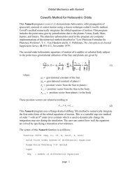
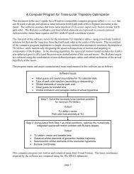
===================program leo2geo_ocs===================transfer time algorithm-----------------------Edelbaum algorithm (non-coplanar orbits)initial guess type------------------linear guess with tangential thrustinggravity model type------------------j2 earth gravity model------------------------beginning of finite burn------------------------sma (km) eccentricity inclination (deg) argper (deg)0.700000000000D+04 0.615067684519D-16 0.285000000000D+02 0.000000000000D+00raan (deg) true anomaly (deg) arglat (deg) period (min)0.206748308333D-14 0.285866456178D+03 0.285866456178D+03 0.971419368695D+02rx (km) ry (km) rz (km) rmag (km)0.191377284137D+04 -.591734870255D+04 -.321285820480D+04 0.700000000000D+04vx (kps) vy (kps) vz (kps) vmag (kps)0.725856076669D+01 0.181305405204D+01 0.984408031306D+00 0.754605384101D+01------------------end of finite burn------------------sma (km) eccentricity inclination (deg) argper (deg)0.420000000000D+05 0.999999999999D-03 0.100000000000D+01 0.360000000000D+03raan (deg) true anomaly (deg) arglat (deg) period (min)0.000000000000D+00 0.423922295262D+02 0.423922295262D+02 0.142768906774D+04rx (km) ry (km) rz (km) rmag (km)0.309960418384D+05 0.282912582669D+05 0.493825749949D+03 0.419689619582D+05vx (kps) vy (kps) vz (kps) vmag (kps)-.207699129982D+01 0.227794898386D+01 0.397617474165D-01 0.308294103563D+01transfer time 15.0823889600487 hoursspacecraft mass 835.576420850925 kilogramspropellant mass 164.423579149075 kilogramsdelta-v 5813.28840908474 meters/secondThe following are typical transfer trajectory, optimal control and orbital element plots for this example.They were created with the Grapher plotting program (www.goldensoftware.com).The first plot is a view of the transfer trajectory from a north pole viewpoint looking down on theequatorial plane. The unit of each trajectory coordinate is Earth radii.page 8

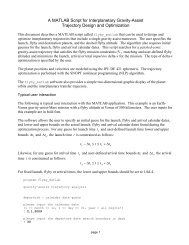
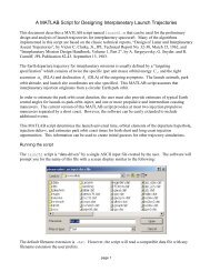
This next plot illustrates the behavior of the pitch and yaw steering angles during the transfer.page 9

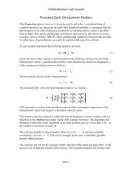
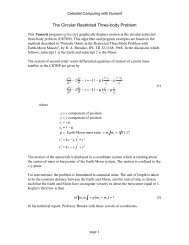
This plot summarizes the inertial right ascension and declination angles for this maneuver.The next three plots illustrate the behavior of the semimajor axis, orbital eccentricity and orbitalinclination of the transfer orbit during the continuous low-thrust maneuver.page 10

page 11

Verification of the optimal control solutionThe optimal control solution determined by the software can be verified by numerically integrating theorbital equations of motion with the optimal control-computed initial park orbit conditions and theoptimal control solution. This is equivalent to solving an initial value problem (IVP) that uses theoptimal unit thrust vector solution. This part of the leo2geo_ocs computer program uses a Runge-Kutta-Fehlberg 7(8) variable step size method to integrate the orbital equations of motion.The following is a summary of the final optimal solution computed using this explicit numericalintegration method.========================================verification of optimal control solution========================================mission orbit state vector and orbital elements-----------------------------------------------sma (km) eccentricity inclination (deg) argper (deg)0.419999999440D+05 0.100000252738D-02 0.999999595528D+00 0.359999478450D+03raan (deg) true anomaly (deg) arglat (deg) period (min)0.359999985471D+03 0.423927660632D+02 0.423922445128D+02 0.142768906488D+04rx (km) ry (km) rz (km) rmag (km)0.309960417074D+05 0.282912586047D+05 0.493825693260D+03 0.419689620884D+05vx (kps) vy (kps) vz (kps) vmag (kps)-.207699129066D+01 0.227794897693D+01 0.397617220168D-01 0.308294102401D+01transfer time 15.0823889600487 hoursspacecraft mass 835.576420851553 kilogramspropellant mass 164.423579148447 kilogramsdelta-v 5813.28840906505 meters/secondCreating an initial guessThe solution to this classic orbit transfer problem requires a good initial guess for the transfer time alongwith a reasonable guess for the dynamic variables during the orbit transfer.Transfer time initial guessThe leo2geo_ocs software implements three options for specifying the transfer time initial guess. Thefirst technique simply integrates the coplanar transfer orbit trajectory using tangential thrusting until thefinal orbit radius is reached. The second method uses Edelbaum’s algorithm. The first method is bestfor coplanar orbit transfers and the second method should be used for non-coplanar orbit transfers. Thethird initial guess option is a user-specified transfer time.For the first technique, the unit thrust vector for tangential steering during the numerical integration isu 0 1 0 T.simply T page 12

The Edelbaum algorithm is described in Chapter 14 of the book Orbital Mechanics by V. Chobotov andthe technical paper, “The Reformulation of Edelbaum's Low-thrust Transfer Problem Using OptimalControl Theory” by J. A. Kechichian, AIAA-92-4576-CP. The original Edelbaum algorithm isdescribed in “Propulsion Requirements for Controllable Satellites”, ARS Journal, Aug. 1961, pp. 1079-1089. This algorithm is valid for total inclination changes i given by 0 i 114.6 and assumes thatthe thrust acceleration magnitude and spacecraft mass are both constant during the orbit transfer.The initial thrust vector yaw angle 0is given by the following expressiontan 0VV0fsin i 2 cosi 2 where the speed on the initial circular orbit is V0 r0and the speed on the final circular orbit isVf rf. In these equations r 0r e h 0is the geocentric radius of the initial orbit, rf re hfis thegeocentric radius of the final orbit, r eis the radius of the Earth and is the gravitational constant of theEarth. The initial altitude is h 0and the final altitude is h f.The total velocity change required for a low-thrust orbit transfer is given byV0sin0V V0cos0tan i 0 2 The total transfer time is given by t V f where f is the thrust acceleration. This is the transfer timeused for the Edelbaum guess option in the leo2geo_ocs software.Dynamic variables initial guessThe dynamic variables at each grid point of the initial guess are determined by setting the initial guessoption INIT(1) = 6 with INIT(2) = 2 within the odeinp subroutine for this aerospace trajectoryoptimization problem. These program options create an initial guess from the numerical integration ofthe equations of motion coded in the oderhs subroutine. The INIT(1) = 6 program option tells theSparse Optimization Suite to construct an initial guess by solving an initial value problem (IVP) with alinear control approximation. The INIT(2) = 2 program option tells the program to use the Dormand-Prince variable step size numerical method to solve the initial value problem.Binary restart file initial guessBinary restart data files can also be used to initialize a leo2geo_ocs simulation. A typical scenario is1. Create a binary restart file from a converged and optimized simulation2. Modify the original input file with slightly different spacecraft characteristics, propulsiveparameters or perhaps final mission targets and/or constraintspage 13

The f subscript indicates values on the user-specified final orbit. This set of constraints or boundaryconditions follows from the orbital element definitions21 cosp a e f e g esin h tan i 2 cosk tan i2 sin These boundary conditions are enforced using lower and upper bounds on the dynamic variables at thefinal time.For final orbits that may be near-circular and/or inclined, the final mission constraints are enforced usingpoint functions. This set of point functions is given byh h h h h hx x f y y f z z fr rsin sinwhere h , h , h are the inertial components of the angular momentum vector, r is the geocentric radiusx y zand is the flight path angle. As noted previously, the f subscript indicates mission values on the userspecifiedfinal orbit.A third program option allows the user to constrain a classical orbital element set consisting of thesemimajor axis, orbital eccentricity and inclination using point functions. This set of mission constraintsisa afe ef i ifAs before the f subscript indicates values on the user-specified final orbit.Bounds on the dynamic variablesThe following lower and upper bounds are applied to the spacecraft mass and the modified equinoctialdynamic variables during the orbital transfer.0.05m m 1.05m1.1p p 0.9p1 f 1 1 g 11 h 1 1 k 10 L 2002fscisc sciffipage 15

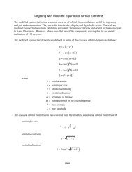
wheremsc iis the initial spacecraft mass, and piis the semiparameter of the initial orbit andpfis thesemiparameter of the final orbit. The upper bound on true longitude L allows for a maximum of 200complete orbits during the transfer.Finally, the components of the unit thrust vector are constrained as follows:Technical discussion1.1 u 1.11.1 u 1.11.1 u 1.1The modified equinoctial orbital elements are a set of orbital elements that are useful for trajectoryanalysis and optimization. They are valid for circular, elliptic, and hyperbolic orbits. These equationsexhibit no singularity for zero eccentricity and orbital inclinations equal to 0 and 90 degrees. However,two components of the orbital element set are singular for an orbital inclination of 180 degrees.The relationship between direct modified equinoctial and classical orbital elements is defined by thefollowing definitionsrtn21 cosp a e f e g esin h tan i 2 cosk tan i 2 sin L wherep a e i L semiparametersemimajor axisorbital eccentricityorbital inclinationargument of periapsisright ascension of the ascending nodetrue anomalytrue longitudeThe relationship between classical and modified equinoctial orbital elements is:psemimajor axis a 2 21 f gorbital eccentricity2 2e f gorbital inclination i 2 tan 1 h 2 k2page 16

argument of periapsis 1 tang f tan1k h1right ascension of the ascending node tan khtrue anomaly L L tan1g f The mathematical relationships between an inertial state vector and the corresponding modifiedequinoctial elements are summarized as follows:position vector r2 cos L cos L 2hk sin L2sr2r 2 sin L sin L 2hk cos Ls2r 2 h sin L k cos L svelocity vector 1 2 sin sin 2 cos 2 s p 1 v 2 cos cos 2 sin 2 s p 2 2h cos L k sin L f h gk s p2 2L L hk L g f hk g2 2L L hk L f ghk fwhere h k s 1 h k2 2 2 2 2 2pr w 1 f cos L g sin LwThe system of first-order modified equinoctial equations of orbital motion are given bydp 2 p pp dt w df p tgf rsin L w 1 cos L f hsin L k cos Ldt w wdg p tf g rcos L w 1 sin L g hsin L k cos Ldt w wpage 17tnn

dhh dt2p s 2wncos Ldkk dt2p s 2wnsin L2dL w 1 pL p hsin L k cos Lndtp w where r, t , nare non-two-body perturbations in the radial, tangential and normal directions,respectively. The radial direction is along the geocentric radius vector of the spacecraft measuredpositive in a direction away from the gravitational center, the tangential direction is perpendicular to thisradius vector measured positive in the direction of orbital motion, and the normal direction is positive inthe direction of the angular momentum vector of the spacecraft’s orbit.The equations of orbital motion can also be expressed in vector form as follows:wheredyy A yP bdt2 p p 0 0 w p p 1p g sin L w 1cos L f h sin L k cos L w w p p 1p f cos L w 1sin L g h sin L k cos L w wA 2p s cos L0 0 2w2p s sin L 0 0 2wp 1 0 0 h sin L k cos L wandb 0 0 0 0 02w p p TThe total non-two-body acceleration vector is given bypage 18

P ˆi ˆi ˆir r t t n nwhere ˆ i , ˆ and ˆrit inare unit vectors in the radial, tangential and normal directions. These unit vectors canbe computed from the inertial position vector r and velocity vector v according toˆ r ˆ r v ˆ ˆ ˆr v rir in it in irr r v r v rFor unperturbed two-body motion, P 0 and the first five equations of motion are simplyp f g h k 0 . Therefore, for two-body motion these modified equinoctial orbital elements areconstant. The true longitude is often called the fast variable of this orbital element set.Propulsive thrustThe acceleration due to propulsive thrust can be expressed asaTT u ˆmTwhere T is the thrust magnitude, m is the spacecraft mass and u ˆT uT ur Tu t Tnis the unit pointingthrust vector expressed in the spacecraft-centered radial-tangential-normal coordinate system. Thecomponents of this unit vector are the control variables.The propellant mass flow rate is determined fromdm Tm dt g IspTwhere g is the acceleration of gravity and Ispis the specific impulse of the propulsive system. Theproduct gIspis also called the exhaust velocity. This differential equation and the modified equinoctialdifferential equations are included in the right-hand-side subroutine required by the software.The spacecraft mass at any mission elapsed time t is given bymass of the spacecraft.mtm mt wheresc imsc iis the initialThe components of the unit thrust vector can also be defined in terms of the in-plane pitch angle andthe out-of-plane yaw angle as follows:u sin u cos cos u cos sinTr Tt TnThe pitch and yaw angles can be determined from the components of the unit thrust vector according topage 19

sin 1uTr1tan uT,nThe pitch angle is positive above the “local horizontal” and the yaw angle is positive in the direction ofthe angular momentum vector of the transfer orbit.The relationship between a unit thrust vector in the Earth-centered-inertial (ECI) coordinate system u ˆT ECIand the corresponding unit thrust vector in the modified equinoctial (MEE) system u ˆT MEEis given byuTtwhereuˆ ˆ ˆ ˆ ˆECI i i i uT r t n TMEEThis relationship can also be expressed asˆ r ˆ r v ˆ ˆ ˆr v rir in it in irr r v r v rrˆˆ ˆ ˆxh r h xx uˆ Quˆ rˆhˆrˆhˆuˆy ˆ ˆ ˆ ˆrzh r hzz TECI TMEE y y TMEEFinally, the transformation of the unit thrust vector in the ECI system to the modified equinoctialcoordinate system is given byFor the case of tangential steeringuˆ Q u ˆTMEETpage 20TECIˆ ˆ ˆ ˆ ˆ ˆ uˆT h r h r h rECI x y zIn the leo2geo_ocs computer program, the components of the inertial unit thrust vector are defined interms of the right ascension and the declination angle as follows:u cos cos u sin cos u sinTECI Tx ECI Ty ECI zFinally, the right ascension and declination angles can be determined from the components of the ECIunit thrust vector according touT u ECI T uy ECI Tx ECI z tan , sin1 1where the calculation for right ascension is a four quadrant inverse tangent operation.T

Gravitational accelerationThe non-spherical gravitational acceleration vector can be expressed asg g ˆi gˆiN N r rwhereandˆiNTeˆ eˆˆi ˆiN N r rTeˆ eˆˆi ˆiN N r re ˆ 0 0 1 TN In these equations the north direction component is indicated by subscript N and the radial directioncomponent is subscript r.The contributions due to a zonal gravity model of order n are as follows:gn kcosRe 'N P2 kJkr k2rnk Rer 2 1 k kr k2rg k P J where RJr e kPkgravitational constantgeocentric distance of the spacecraftequatorial radius of the Earthgeocentric latitudezonal gravity coefficientthk order Legendre polynomialFor a zonal only Earth gravity model, the east component is identically zero.Finally, the zonal gravity perturbation contribution isa gQ Tgwhere Q ˆ ˆ ˆ ir it in .For J2effects only, the three components are as follows:page 21

23JR122hsin L k cos LeJ 1242 22r2r 1h k2J2t212JR2 e 4r 1h khsin L k cos Lhcos L k sin L2 22J2n2 21 h k hsin L k cos L26JR2 e 4r 1h k2 22These are the equations implemented in this computer program.page 22

Algorithm resourcesAn Introduction to the Mathematics and Methods of Astrodynamics, Richard H. Battin, AIAA EducationSeries, 1987.Analytical Mechanics of Space Systems, Hanspeter Schaub and John L. Junkins, AIAA EducationSeries, 2003.Spacecraft Mission Design, Charles D. Brown, AIAA Education Series, 1992.Orbital Mechanics, Vladimir A. Chobotov, AIAA Education Series, 2002.“Optimal Low Thrust Trajectories to the Moon”, John T. Betts and Sven O. Erb, SIAM Journal onApplied Dynamical Systems, Vol. 2, No. 2, pp. 144-170, 2003.“A Set of Modified Equinoctial Orbital Elements”, M. J. H. Walker, B. Ireland and J. Owens, CelestialMechanics, Vol. 36, pp. 409-419, 1985.“On the Equinoctial Orbital Elements”, R. A. Brouke and P. J. Cefola, Celestial Mechanics, Vol. 5, pp.303-310, 1972.“Optimal Interplanetary Orbit Transfers by Direct Transcription”, John T. Betts, The Journal of theAstronautical Sciences, Vol. 42, No. 3, July-September 1994, pp. 247-268.“Using Sparse Nonlinear Programming to Compute Low Thrust Orbit Transfers”, John T. Betts, TheJournal of the Astronautical Sciences, Vol. 41, No. 3, July-September 1993, pp. 349-371.“Equinoctial Orbit Elements: Application to Optimal Transfer Problems”, Jean A. Kechichian, AIAA90-2976, AIAA/AAS Astrodynamics Conference, Portland, OR, 20-22 August 1990.page 23

APPENDIX AContents of the Simulation Summary and CSV FilesThis appendix is a brief summary of the information contained in the simulation summary screendisplays and the CSV data files produced by the leo2geo_ocs software.The simulation summary screen display contains the following information:sma (km) = semimajor axis in kilometerseccentricity = orbital eccentricity (non-dimensional)inclination (deg) = orbital inclination in degreesargper (deg) = argument of perigee in degreesraan (deg) = right ascension of the ascending node in degreestrue anomaly (deg) = true anomaly in degreesarglat (deg) = argument of latitude in degrees. The argument of latitude is the sum oftrue anomaly and argument of perigee.period (min) = orbital period in minutesrx (km) = x-component of the spacecraft’s position vector in kilometersry (km) = y-component of the spacecraft’s position vector in kilometersrz (km) = z-component of the spacecraft’s position vector in kilometersrmag (km) = scalar magnitude of the spacecraft’s position vector in kilometersvx (km/sec) = x-component of the spacecraft’s velocity vector in kilometers per secondvy (km/sec) = y-component of the spacecraft’s velocity vector in kilometers per secondvz (km/sec) = z-component of the spacecraft’s velocity vector in kilometers per secondvmag (km/sec) = scalar magnitude of the spacecraft’s velocity vector in kilometers persecondtransfer time = total thrust duration in hoursfinal mass = final spacecraft mass in kilogramspropellant mass = expended propellant mass in kilogramsthrust duration = maneuver duration in secondsdelta-v = scalar magnitude of the accumulated delta-v in meters/secondsThe delta-v is determined using a cubic spline integration of the thrust acceleration data at eachcollocation node.The comma-separated-variable disk file is created by the odeprt subroutine and contains the followinginformation:time (hrs) = simulation time since ignition in hourspage 24

time (days) = simulation time since ignition in dayssemimajor axis (km) = semimajor axis in kilometerseccentricity = orbital eccentricity (non-dimensional)inclination (deg) = orbital inclination in degreesargument of perigee (deg) = argument of perigee in degreesraan (deg) = right ascension of the ascending node in degreestrue anomaly = true anomaly in degreesperiod (min) = orbital period in minutesmass (kg) = spacecraft mass in kilogramsT/W = thrust-to-weight ratioyaw = thrust vector yaw angle in degreespitch = thrust vector pitch angle in degreesperigee altitude = perigee altitude in kilometersapogee altitude = apogee altitude in kilometersut-radial = radial component of unit thrust vectorut-tangential = tangential component of unit thrust vectorut-normal = normal component of unit thrust vectorsemi-parameter = orbital semiparameter in kilometersf equinoctial element = modified equinoctial orbital elementg equinoctial element = modified equinoctial orbital elementh equinoctial element = modified equinoctial orbital elementk equinoctial element = modified equinoctial orbital elementtrue longitude = true longitude in degreesrx (er) = x-component of the spacecraft’s position vector in Earth radiiry (er) = y-component of the spacecraft’s position vector in Earth radiirz (er) = z-component of the spacecraft’s position vector in Earth radiifpa (deg) = flight path angle in degreesdvacc (mps) = accumulative delta-v in meters per secondpage 25

APPENDIX BTypical Sparse Optimization Suite Configuration FileThe leo2geo_ocs computer progran can read and use a user-defined configuration file. A descriptionof each element in this file can be found in the INOCS routine in section 6.2, Subprograms for OptimalControl, and the INSNLP routine in Section 2.2, Subprograms for Optimization of the SparseOptimization Suite user’s manual. Please note that the leo2geo_ocs software can read and use asubset of the information in this file. For example, a subset configuration file might contain only thefollowing information;ODETOL=0.1D-06INSNLP:IOFLAG=5SOCOUT=I4K4The following is a typical “full version” configuration file created during the execution of theleo2geo_ocs software.AEQTOL=0.1000000000000000D-02DTAUX=0.0000000000000000D+00OBJCTL=0.1000000000000000D-04ODETOL=0.1000000011686097D-06PGDCTL=0.1000000000000000D-02PRTMSD=0.1490116119384766D-07PRTMXD=0.1000000000000000D-02PRTSFD=0.1000000000000000D-04QDRTOL=0.1000000000000000D-02RESTOL=0.1000000000000000D-04SMLTOL=0.1490116119384766D-10TOLJSD=0.1000000000000000D-05TOLM5A=0.1490116119384766D-07TOLM5R=0.1490116119384766D-07IDSCPH=0IDSCND=0IDSCVR=0IDSCFN=0IDTSFD=-1IPFAUX=0IPFSFD=0IPRSFD=1IPGRD=0IPNLP=10IPODE=0IPUAUX=0IPUOCP=6IRSTRT=2ISCALE=0ISFHES=41ISFINP=42ISFRST=43ISFSCL=44ITSWCH=2M5DTYP=0MITODE=20MTSWCH=-1MXDATA=0MXPARM=10MXPCON=20MXSTAT=20MXTERM=50NPTAUX=100NSSWCH=-1SOCOUT=A0B0C0D0E0F0G0H0I0J2K0L0M0N0O0P0Q0R0S1T0U0V0W0X0Y0Z0SPRTHS=SPARSENLPALG=SNLPMNNLPOMR=MKEYDPL=.lueiLUEpage 26

page 27RHSTMP=RHSTMPLTRSTFIL=hyper1.rsbinSCLFIL=scalewgt.filINSNLP:ALFLWR=0.0000000000000000D+00INSNLP:ALFUPR=0.1000000000000000D+01INSNLP:CONTOL=0.1490116119384766D-07INSNLP:EPSRLF=0.1490116119384766D-07INSNLP:OBJTOL=0.9999999747378752D-05INSNLP:PGDTOL=0.1000000000000000D-04INSNLP:SLPTOL=0.9000000000000000D+00INSNLP:SFZTOL=0.1000000000000000D-01INSNLP:TOLFIL=0.2000000000000000D+01INSNLP:TOLKTC=0.1110953834938985D+26INSNLP:TOLPVT=0.1000000000000000D-02INSNLP:IHESHN=0INSNLP:IOFLAG=5INSNLP:IOFLIN=-1INSNLP:IOFMFR=0INSNLP:IOFPAT=0INSNLP:IOFSHR=0INSNLP:IOFSRC=0INSNLP:IPUDRF=0INSNLP:IPUFZF=0INSNLP:IPUMF1=11INSNLP:IPUMF2=12INSNLP:IPUMF3=13INSNLP:IPUMF4=14INSNLP:IPUMF5=15INSNLP:IPUMF6=16INSNLP:IPUMF7=17INSNLP:IPUNLP=6INSNLP:IPUSTF=0INSNLP:IRELAX=1INSNLP:ITDRQP=-1INSNLP:ITFZQP=-1INSNLP:IT1MAX=20INSNLP:JACPRM=0INSNLP:LYNFNC=0INSNLP:LYNOUT=0INSNLP:LYNPLT=0INSNLP:LYNPNT=101INSNLP:LYNVAR=0INSNLP:MAXLYN=5INSNLP:MAXNFE=50000INSNLP:MNSAME=2INSNLP:NEWTON=0INSNLP:NITMAX=1000INSNLP:NITMIN=0INSNLP:NORMAL=0INSNLP:ALGOPT=FMINSNLP:KTOPTN=SMALLINSNLP:QPOPTN=SPARSEINSNLP:BIGCON=-0.1000000000000000D+01INSNLP:FEATOL=0.1000000000000000D-01INSNLP:PMULWR=0.1000000000000000D+00INSNLP:PTHTOL=0.1000000000000000D+02INSNLP:RHOLWR=0.1000000000000000D+03INSNLP:IMAXMU=10INSNLP:MUCALC=3INSNLP:MXQPIT=1