CELESTIAL COMPUTING - Orbital and Celestial Mechanics Website

ISSN 1044 - 9825CELESTIALCOMPUTINGA Journal for Personal Computers and Celestial MechanicsVolume 4 Number 1 Winter 1991-92Feature ArticleEphemerides for Physical Observations Page 1Fundamental AstronomyA Computer Implementation of Newcomb's Solar Theory Page 9Applied AstrodynamicsPredicting Lunar Eclipses of Earth Satellites Page 11Symbolic ComputingSymbolic Computing and Graphics with Mercury Page 14Recreational ComputingA Mercator Graphics Display of Earth Satellite Groundtracks Page 20Numerical MethodsA Computer Method for Solving Systems of Nonlinear Equations Page 24Celestial Book ReviewAstronomy on the Personal Computer Page 27Celestial Software ReviewProgram ASTRONOMY LAB Page 29Copyright © 1991 by David Eagle. All rights reserved.

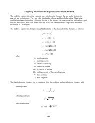
Vol.4 • Na.l Gele&tiat Gomputinq Wlnten 1991-92FEATURE ARTICLEMethods for calculating a physical ephemeris of the Sun and planets is the topicfor this FEATURE ARTICLE. A physical ephemeris represents the orientation andillumination of the apparent disk of a celestial body as seen by an observer onthe Earth. This information can be used by the astronomer to gather and reduceobservations of visible surface markings on a planet or sunspots on the Sun.These measurements can be used to determine the planetographic or heliographiccoordinates of physical features and unusual phenomena.An excellent technical discussion about physical ephemerides can be found inChapter 11 of "Ephemerides for Physical Observations of the Sun, Moon, andPlanets", in the Explanatory Supplement to the Ephemeris, 1964. Additionalmaterial can also be found in Sections 17.4-17.8 of Chapter 17 of Green's book,Spherical Astronomy.The companion floppy disk for this issue contains an interactive QuickBASICcomputer program called PEPHEM. BAS which provides the following physicalephemeris information about the Suno Position angle of the rotation axiso Heliographic latitude of the central pointo Heliographic longitude of the central pointand the following illumination and rotation data for the planets:o Apparent diametero Phase angleo Phaseo Defect of illuminationo Visual magnitudeo Right ascension and declination of the rotation axiso Position angle of the rotation axiso Orientation of the prime meridianThe position vectors of the Sun and planets are determined in program PEPHEMusing the methods described in "Low-precision Formulae for Planetary Positions".Most of the astronomical constants required to compute physical ephemerides istaken from the Supplement to the Astronomical Almanac 1984. The informationdescribed in this supplement can also be found in "Report of the lAU/IAG/COSPARWorking Group on Cartographic Coordinates and Rotational Elements of the Planetsand Satellites: 1985", Celestial Mechanics 39 (1986) 103-113.

Vol.4 • No.. I %ele&tial Computing Wlnten 1991-92Physical Ephemerides of the SunProgram PEPHEM uses a combination of Chapters 18 and 41 of Astronomical Formulaefor Calculators by Jean Meeus to compute a physical ephemeris of the Sun. Thesoftware calculates the following elements of a solar physical ephemeris:PBL= Position angle of the rotation axis= Heliographic latitude of the central point= Heliographic longitude of the central pointThe position angle P of the northern extremity of the Sun* s axis of rotation ismeasured positive eastwards from the North point of the solar disk. The northpoint of the solar disk is determined by the the equator and equinox of date.Heliographic coordinates can be used to define the position of sunspots or otherpoints on the surface of the Sun. Heliographic latitudes range between ± 90degrees and are defined with respect to the solar equator which is inclined atan angle of 7 degrees, 15 minutes with respect to the ecliptic. Heliographiclongitudes range between 0 and 360 degrees and are measured with respect to thesolar meridian which passed through the ascending node of the solar equator onthe ecliptic on January 1, 1854 at Greenwich mean noon.The time argument for the solar ephemeris calculations is the number of Juliancenturies given by the expressionT = JED ~ 24150201 36525 11jwhere JED is the Julian Ephemeris Date of interest.The geometric mean longitude, mean anomaly and right ascension of the ascendingnode of the Sun are calculated with the next three equations:L = 279^69668 + 36000*76892 T + 0*0003025 T2 (2)M = 358°47583 + 35999*04975 T - O.°000150 T2 - 0*0000033 T3 (3)Q = 259*18 - 1934*142 T (4)The true longitude of the Sun is given byA0 = L + C (5)where C is called the equation of the center and is calculated withC = (1*91946 - 0*004789 T - 0*000014 T2) sin M+ (0*020094 - 0*0001 T) sin 2M + 0*000293 sin 3M (6)

Vol.4 • No.. I Gele&bial Waniputiru), Wlnten 1991-92The apparent longitude of the Sun consists of the true longitude and correctionsfor aberration and nutation as follows:A = A - (L00569 - CL00479 sin Q (7)a GThe actual physical ephemeris computations begin with6 = ^^5 (JED - 2398220) (8)Zo. JoThe inclination of the equator of the Sun relative to the ecliptic plane isI = 7.25°and the longitude of the ascending node of the solar equator isK = 74°3646 + 1.395833 T (9)The calculations continue withtan X = - cos A7 tan etan Y = - cos(A - K) tan Iwhere e is the obliquity of the ecliptic and A' is the Sun* s apparentcorrected for nutation.(lOa)(lOb)longitudeThe mean obliquity is determined frome = 23°452295 - CL0130125 T - 0^00000164 T2 + 0*000000503 T3 (11)and with the correction for nutation becomese = c + 0°00256 cos Q (12)oFinally, the position angle of the axis of rotation isP = X + Y (13)The heliographic latitude of the central point of the Sun's disk isB = sin'MsinU - K) sin l] (14)and the heliographic longitude isLQ = T) - 6 (15)where7? = ATAN3(- sin(A - K) cos I, - cos(A - K))

Vol.4 • Ma. 1 GeleAtial ^omputinq, Wlnten 1991-92Physical Ephemerides of the PlanetsMany of the physical ephemerides calculations for the planets described in thissection are based on algorithms described in Chapter 6 of Practical EphemerisCalculations by Oliver Montenbruck, Springer-Verlag, 1989.Apparent Diameter of a Planet's DiskThe apparent diameter of a planet as viewed from the Earth is given by(2 tan s %-- (16)A *wheresoA= semidiameter at 1 Astronomical Unit= geocentric distance of the planet (AU's)Position Angle of a Planet's Axis of RotationThe angle between the north direction and the plane through a planet's rotationaxis is called the position angle of the axis of rotation. The position angle Pis determined with an ATAN3 calculation of the following two equations:sin P = cos d sin(a - a) (17a)a acos P = sin d cos d - cos d sin d cos(a - a) (17b)a a aP = ATAN3(sin P, cos P) (18)where a and d are the rotation axis coordinates and a and d are the geocentrica aequatorial coordinates of the planet. The calculation of the rotation axisright ascension and declination is described below in the section "Orientationof the Rotation axis of a Planet".Phase Angle of a Planet's DiskThe phase angle is the angle between the Sun and the Earth as viewed from aplanet. It can be determined with a equation of the form-if A2 - r2- R2= cos — - (19)whereA = geocentric distance of the planetr = heliocentric distance of the planetR = heliocentric distance of the Earth

Vol.4 • Na.l ^eie^tial gom/utOag Winten 1991-92For our purposes the phase function is assumed to be a linear function of thephase angle. The phase function is evaluated in program PEPHEM using the linearinterpolation subroutine INTERP1 which was described in the NUMERICAL METHODScolumn of the Fall 1991 issue of Celestial Computing.The common logarithm required for these visual magnitude calculations is codedwith the following QuickBASIC function:LOGIO(X) = LOG(X) / LOG(lOtt)Orientation of the Rotation Axis of a PlanetThe right ascension and declination angles of a planet's rotation axis can bedetermined from equations of the forma = a + a T + Aa T (23a)N, i N, i N, i6 = 6 +6 T + A6 T (23b)N, i N, i N, iThe first two terms of the orientation angles are the coordinates with respectto the J2000 equinox. The A term is a correction to bring the angles to thecurrent Earth equinox and equator. The time argument T is the number of Juliancenturies from J2000 and is determined from the Julian Ephemeris Date (JED) as= JED - 24515451 36525 l^jFor example, the two orientation calculations for Mars are

Vol.4 • No.. I %ele&tlal ^omputinq Wlnten 1991-92Furthermore, all the zones of Saturn and Jupiter do not rotate at the same speedand prime meridians are defined for these two planets in several systems. Thesesystems are defined with respect to regions of the planet as follows:System I - rotation in the equatorial region of the planetSystem II - rotation in the higher latitudes of the planetSystem III - rotation based on radio signals from the planetThe location of a planet's prime or null meridian is determined with an equationof the form:W = W + AW T (26)J2000where W is the meridian orientation with respect to the J2000 epoch and isJ2000determined with an equation which looks likeW = W + W d (27)JOOO 0In this equation d = JED - 2451545 and is the number of days relative to January1, 2000. The time argument T of Eq. (26) is calculated using Eq. (24). It canalso be determined from T = d/36525.For example, the prime meridian calculation for Venus is simplyW = 159^91 - 1^4814205 d + l.°436 T (28)and for the three systems for Jupiter they areSystem I W = 67°10 + 877*900 d + 1°291 T (29a)System II W = 43°30 + 870*270 d + 1*291 T (29b)System III W = 284°95 + 870°536 d + 1°291 T (29c)Program NotesThe program will begin by prompting you for the calendar date and time at whichto compute the physical ephemeris. The software is valid between 1670 and 2230A. D. Be sure to input all the digits of the calendar year. The user may inputeither Ephemeris or Universal time and the software will make the properconversions. The software will then display a menu of the planet names and theSun and ask you to select one.The software will display the calendar and Julian Ephemeris Dates and theUniversal and Ephemeris Times. For planets the illumination characteristics aredisplayed followed by the rotation data. The phase is printed as a fraction andcan be converted to percent by multiplying by 100.7

Vol.4 • Na.l ^el&dial ^omputinq Wlnten 1991-92The following are typical screen displays from program PEPHEM. They illustratethe physical ephemerides for Mars and the Sun at 20 hours Universal Time onJanuary 1, 1992.Program PEPHEM< Ephemerides for Physical Observations of the Sun and Planets >Calendar date January 1, 1992Universal Time 20 hrs 00 min 00 secEphemeris time 20 hrs 01 min 33 secJulian Ephemeris Date 2448623.334406Ephemeris for Physical Observations of Mars< Illumination Characteristics >Apparent diameter3.88 arc secondsPhase angle 11° 19' 38"Phase 0.990Defect of illumination0.04 arc secondsVisual magnitude 1.410< Rotation Characteristics >Right ascension of the rotation axis 317° 37' 36"Declination of the rotation axis 52° 51' 28"Position angle of the rotation axis 29° 087 07"Orientation of the prime meridian 267° 347 17"Ephemeris for Physical Observations of the SunPosition angle of the rotation axis 1° 59' 24"Heliographic latitude of the central point - 3° 037 30"Heliographic longitude of the central point 43 55' 10"

Vol. 4 • Na.l Gele&tial Wcwputinq, Winten, 1991-92FUNDAMENTAL ASTRONOMYIn this session of FUNDAMENTAL ASTRONOMY we present a QuickBASIC implementationof Simon Newcomb's classic solar ephemeris. The SOLAR.BAS program was ported toQuickBASIC from a FORTRAN version provided to Celestial Computing by Dr. BrianMarsden of the Smithsonian Astrophysical Observatory. We would like to thankDr. Marsden for his help and permission to offer this software to our readers.Simon Newcomb's solar theory first appeared in-Volume 6 of Astronomical Papersprepared for the use of the American Ephemeris and Nautical Almanac published in1898 with the title "Tables of the Motion of the Earth on its Axis and Aroundthe Sun". It appears that work on this ephemeris began around 1877 andaccording to Newcomb, "The prosecution of such a work as this required, in someinstances, a grade of technical ability above that of the routine computer".The "routine computer" he talks about is a person, not an electronic machine. Adiscussion and computational outline of Newcomb*s solar theory can also be foundin Section 4.1.2 of Chapter 4 of Oliver Montenbruck' s book, Practical EphemerisCalculations, Springer-Verlag, 1989.Program SOLAR calculates the geocentric, rectangular position vector of the Sunwith respect to the mean equator and equinox of 1950. It consists of a shortdriver program which demonstrates how to call a subroutine which performs theactual computations.If you incorporate SOLAR into programs you write, please note that it uses thefollowing type declarations for all constants, variables and function names:DEFINT I-NDEFDBL A-H, 0-ZThe main subroutine has the following syntax:SUB SOLAR(DJ, RO) STATICwhere DJ is passed to the subroutine as the Julian Ephemeris Date of interestand R() is a 1 by 3 array returned by the subroutine as the geocentric positionvector. The R() vector has the units of Astronomical Units.The SOLAR subroutine also requires numeric data which is coded into a series ofQuickBASIC DATA statements at the end of the driver program. This data isloaded into a two-dimensional double precision array named Z with the followingFOR-NEXT statements:FOR XK = 1 TO 121FOR I = 1 TO 8READ Z(I, XK)NEXT INEXT XK

Vol.4 • No.. I ^eletitial ^ompidlng, Winten 1991-92The Z array is dimensioned and passed to the SOLAR subroutine with the followingglobal statementDIM SHARED Z(8, 121)This statement must appear in the main program following all DECLARE statements.Program NotesThe software will prompt you for the calendar date and Ephemeris Time. Be sureto include the full calendar year as part of your input. The time should beinput in 24 hour format.The output from program SOLAR consists of the Julian Ephemeris Date and thegeocentric rectangular coordinates of the Sun. The coordinates are with respectto the mean equator and equinox of 1950. They are printed in both AstronomicalUnits and kilometers. The conversion factor from AU* s to kilometers used inSOLAR is 149597870.66 kilometers per Astronomical Unit.The following is a typical display generated by program SOLAR.GEOCENTRIC RECTANGULAR COORDINATES OF THE SUNCalendar Date February 1, 1983Ephemeris Time 0 hr 0 min 0 secJulian Ephemeris Date 2445366.5< Position Vector - Mean Equator and Equinox of 1950 - AU's >. 6476459873484262 -. 6812380109936663 -2953863900977958< Position Vector - Mean Equator and Equinox of 1950 - kilometers >96886460.64881785 -101911755.8573062 -44189174.98057436The Astronomical Almanac for the year 1983 tabulated the Sun's position vectorin Astronomical Units at 0 hours ET as follows:.6476460 -.6812380 -.2953864These numbers agree quite well with a solar ephemeris which was developed almostone hundred years ago!10

Vol.4 • Na.l GeleAtiat Gamputinq Wlnten 1991-92APPLIED ASTRODYNAMICSThis edition of APPLIED ASTRODYNAMICS describes a QuickBASIC computer programcalled LESAT which can be used to determine lunar eclipses of Earth satellites.A technical discussion of this problem can be found in Chapter 6 of Methods ofAstrodynamics by P. R. Escobal. Lunar eclipses of satellites can affect suchthings as spacecraft power, viewing conditions, and radio communications.Program LESAT uses a modification of the method of calculating solar eclipsesdescribed in the FEATURE ARTICLE of the Spring 1990 issue of Celestial Computingto determine possible lunar eclipses of Earth satellites. The calculationswhich pertain to an Earth observer are simply replaced with an Earth satellite.The following is a short discussion about the minor changes to the software.The angle 7) of Figure 1 is calculated with the equation. -117 = sindR m-s(1)where Rm-sis distance from the Moon to the satellite.The umbra angle at the satellite's distance is determined from. . -i ( d sin 6 1 ,_.$ = sin -g (2)^ m-s 'The separation angle between the shadow axis and the Earth satellite at any timeduring the umbra or penumbra eclipse is:-if" " ^ = cos U • U (3)I m-s m-sun IProgram NotesProgram LESAT will begin by prompting you to input the initial calendar date,universal time, and the total simulation period in days. The program is validbetween the calendar years 1670 and 2070. The software will then request thegeocentric classical orbital elements of the satellite of interest.After all the program requests have been provided, the user is asked if he orshe would like to print the simulation definition. This feature allows you tomake a copy of the information which initialized program LESAT.The program will provide the calendar date, universal time, and distances atentrance and exit of the satellite relative to each part of the Moon's shadow.The screen display includes the geocentric and selenocentric distances of theEarth-orbiting satellite in the units of kilometers.11

Vol. 4 • Na. 1 Winten 1991-92The following is typical data generated by program LESAT.conditions for a geosynchronous satellite.It illustrates shadowProgram LESAT< Lunar Eclipse of Earth Satellites >Initial calendar dateInitial universal timeSemimajor axisEccentricityInclinationArgument of perigeeRight ascension of the ascending nodeTrue anomaly( km )( degrees )( degrees )( degrees )( degrees )July 12, 19915 h 00 m 00 s42164.5000.0000000.0000.0000.000291.450Calendar dateUniversal timeJulian DateEnter Penumbra ShadowEarth-to-satellite distance (km)Moon-to-satellite distance (km)Calendar dateUniversal timeJulian DateEnter Umbra ShadowEarth-to-satellite distance (km)Moon-to-satellite distance (km)Calendar dateUniversal timeJulian DateExit Umbra ShadowEarth-to-satellite distance (km)Moon-to-satellite distance (km)Calendar dateUniversal timeJulian DateExit Penumbra ShadowEarth-to-satellite distance (km)Moon-to-satellite distance (km)December 6, 19914 h 15 m 00 s2448596.67742164.500438655.060December 6, 19914 h 29 m 49 s2448596.68742164.500438748.720December 6, 19914 h 32 m 11 s2448596.68942164.500438751.102December 6, 19914 h 47 m 00 s2448596.69942164.500438687.19612

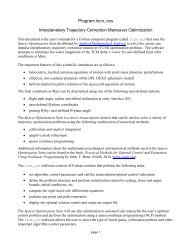
Vol. 4 • Na.l Computing, Wlnten 1991-92The following is a software tree diagram for the LESAT.BAS computer program. Itillustrates the hierarchy of the program flow and subroutine dependencies. Thefirst occurrence of a QuickBASIC subroutine or function also includes a shortcomment describing its purpose. As can be seen from the diagram, most of theprocessing is controlled by the ECLIPSE subroutine. This subroutine performsthe search for possible eclipses and calls 'the appropriate subroutines tocalculate the actual eclipse conditions.MAIN-ATAN3 (four quadrant inverse tangent)-ECLIPSE (search for eclipse)-ASIN (inverse sine)-BMINIMA (bracket minima subroutine)1 OFUNCTION (objective function)ACOS (inverse cosine)I ASINATAN3MODULO (modulo 2 TT)-SUN.MOON (solar/lunar ephemeris)MODULO-R2R (revolution to radians)-RASC.DECL (right ascension/declination)ASINATAN3-BROOT (bracket root)I OFUNCTION-GDATE (calendar date)1 HRS2HMS$ (convert hours to hms string)1 RPAD$ (pad string)-MINIMA (find function minima)I OFUNCTION-PRINT1 (print results)1 KEYCHECK (check user response)-ROOT (find function root)I OFUNCTION-WORKING (print message)HRS2HMS$fLIAN (Julian Date)KEYCHECKCHECK[ODULOT.INIT (calculate perturbations)-WORKINGFigure 1Software Tree Diagram13

Vol.4 • No,. I Gele&tlal Gomputlriq, Wlnten 1991-92SYMBOLIC COMPUTINGThis session of SYMBOLIC COMPUTING demonstrates how to use Mercury to performsymbolic computations and display graphics. Symbolic computing can be a verypowerful and useful tool which provides insight into many complex problems. Theability to display graphics can also help us verify assumptions and conclusions.The Mercury software supports a variety of IBM-PC and true compatible graphicsmodes and printers.To illustrate these Mercury features we revisit the problem of optimal impulsiveorbital transfer between inclined circular orbits once more. This topic wasaddressed in the APPLIED ASTRODYNAMICS column of the Spring 1989 issue ofCelestial Computing. Let's begin with a quick review of the important equationswhich define this problem.The delta-velocity impulse required for the first impulse is given by:AV = V / 1 + H2 - 2 H cos 6 (1)i ic V i i iThe delta-velocity increment required for the second impulse is given by:AV = V / H2 + H2 H2- 2 H2 H cos 9 (2)l c V 2 2 3 2 3 2The total delta-V required for the transfer is simply the sum of Eqs. (1) and (2)as follows:AV = V / 1 + H2 - 2 H cos 6t 1 c V 1 1 1where+ V / H2 + H2 H2- 2 H2 H cos 0 (3)Ic V 2 2 3 23 26 = plane change angle of the initial orbit6 = plane change angle of the final orbitV = -^— = local circular velocityic / r yV ijut= gravitational constantThe total plane change angle of the transfer is given by:e = e + e (4)14

Vol. 4 • Ma. 1 ^eie&tijal SompuUag Winten 1991-92The normalized radii in the equations above are determined from the following:(5a)(5b)(5c)where r is the radius of initial circular orbit and r is the radius of theiffinal circular orbitThe floppy disk for this issue contains a Mercury equation file called GIOTA1which graphically displays the individual and total delta-V required as afunction of each plane change angle. Let's talk about how to use Mercurygraphics by examining the following equation file listing:Program "GIOTAl" October 5, 1991Impulsive Orbital Transfer Analysis with GraphicsThis Mercury program graphically displays therelationships between delta-V and inclinationfor optimal impulsive orbital transfer betweeninclined circular Earth orbits.******************^^Inputhi = initial circular orbit altitude ( kilometers )hf = final circular orbit altitude ( kilometers )it = total plane change angle ( degrees )Outputgraphics display of(1) first impulse delta-V vs first plane change angle(2) second impulse delta-V vs second plane change angle(3) total delta-V vs first plane change angle(4) total delta-V vs second plane change angledefine astrodynamic constants and conversion factormu = 398600.4 ; gravitational constant ( km^3/sec^2 )15

Vol. 4 • Na. 1 %ele&tial go/nputtog Winten, 1991-92req = 6378. 14 ; earth equatorial radius ( km )dtr = pi/180 ; degrees to radians; ******************* user inputs *******************; initial and final orbit altitudes ( kilometers )hi = 277.8hf = 35786; total plane change angle ( degrees )it = 28.5; calculate initial and final orbit radius ( kilometers )ri = req + hirf = req + hf; calculate "local circular velocity" of initial orbit (mps)vie = 1000*SQRT(mu/ri); calculate "normalized" radiihi = SQRT(2*rf/(rf+ri))h2 = SQRT(ri/rf )h3 = SQRT(2*ri/(rf+ri)); define delta-V versus inclination relationshipsdvl(il) := vlc*SQRT(l+hl"2-2*hl*COS(dtr*il))dv2(i2) := vlc*SQRT(h2~2*h3"2+h2"2-2*h2"2*h3*COS(dtr*i2))dvtl(il) := vlc*(SQRT(l+hl~2-2*hl*COS(dtr*il))+ SQRT(h2"2*h3~2+h2"2-2*h2"2*h3*COS(dtr*(it-il ) )dvt2(i2) := vlc*(SQRT(l+hl"2-2*hl*COS(dtr*(it-i2) ) )+ SQRT(h2~2*h3"2+h2"2-2*h2"2*h3*COS(dtr*i2))); ********** generate graphics **********; specify thin lineGSTYLE 1; plot main title and subtitleTITLE "Delta-V Vs Inclination"SUBTITLE "(Impulsive Orbital Transfer)"; x-axis titleXLABEL "INCLINATION (deg)"16

Vol. 4 • Ha. I ^eie&tiaA ^omputirvq Winten 1991-92; y-axis titleYLABEL "DELTA-V (mps)"; define X-axis plot boundsGBOUNDS 0, 30; plot 100 X-Y data pointsGPOINTS 100; display legendLEGEND; plot delta-V as a function of inclinationPLOT dvtl, dvt2, dvl, dv2The first part of this file defines several constants and the altitudes andplane change of the orbit transfer. The equations to be plotted are defined inthe statements which begin with dvl(il) = vlc*SQRT(l+hl/v2-2*hl*COS(dtr*il)).These statements define the functions we would like to plot by declaring them asfunctions of a specific inclination angle. For this example we have elected toplot both the individual and total delta-V*s as functions of plane change anglesbetween 0 and 30 degrees.The actual graphic statements begin in the section "generate graphics". It ishere that we define the kind of line to use for plotting (GSTYLE), the title andaxes labels (TITLE, SUBTITLE, XLABEL, YLABEL) and the independent variableplotting bounds (GBOUNDS). We can also tell Mercury how many data points togenerate (GPOINTS) and exactly which functions to plot (PLOT). For users withcolor displays a "color" legend for each plot can be displayed with the MercuryLEGEND command.To begin the graphic computations, type Solve from the main Mercury menu andthen select the Graph menu after the output window appears. The Solve functionactually generates the graphic data points requested by the user. Within theGraph menu are commands for viewing the graphics on your monitor (View) andprinting the results on a printer (Print).An examination of the plots of total delta-V versus each plane change anglereveals that the total delta-V passes through a minimum on each plot. Thishelps to verify the optimum solution found by the original IOTA equation file.The next report file listing demonstrates how to use Mercury to perform symboliccomputing. For this example we will use the Mercury deriv function tosymbolically compute the partial derivatives of the delta-V functions withrespect to the individual plane change angles. ' Partial differentiation is theprocess of differentiating a multiple-variable function with respect to a singlevariable while holding the others fixed. The partial derivative can be thoughtof as the sensitivity of a function to a particular variable.17

Vol.4 • Na.l ^eie^Unl Sompoiing Wirvtesi 1991-92= Problem: C:\CCV4N1\GIOTA2.EKA —Program "GIOTA2" October .14, 1991Impulsive Orbital Transfer Analysis with GraphicsThis program demonstrates the symbolic computingcapability of Mercury. The partial derivatives oftotal delta-V and versus the two inclination changesfor the problem of optimal impulsive orbital transferbetween inclined circular Earth orbits are computed.******************^define total impulsive delta velocity as a functionof the first and second inclinations, respectively.dvtl(il) := vlc#sqrt(l+hl"2-2*hl*cos(il))+vlc*sqrt(h2"2#h3"2+h2"2-2*h2"2*h3*cos(it-il))dvt2(i2) := Vlc#sqrt(l+hl"2-2#hl*cos(it-i2))+vlc*sqrt(h2"2*h3"2+h2"2-2*h2"2*h3*cos(i2)); compute symbolic derivatives of total delta-V with; respect to each inclination.ddvtdil = deriv(dvtHil), il)ddvtdi2 = deriv(dvt2(i2), i2)= Solution =Variables:11 = UNDEFINEDvie = UNDEFINEDhi = UNDEFINEDh2 = UNDEFINEDh3 = UNDEFINEDit = UNDEFINED12 = UNDEFINEDddvtdil = vlc*(-2*hl*(-SIN(il)))*0.5/SQRT(l+hl"2-2*hl*COS(il))+vlc*(-2*h3*h2"2*SIN(it-il))*0.5/SQRT(h2~2*h3~2+h2"2-2*h3*h2"2*COS(it-il))= NO SOLUTIONddvtdi2 = vlc#(-2#hl#SIN(it-i2))*0.5/SQRT(l+hl"2-2*hl*COS(it-i2))+vlc*(-2*h3*(-SIN(i2))*h2"2)*0.5/SQRT(h2"2*h3~2+h2"2-2#h3#h2"2*COS(i2))= NO SOLUTIONResiduals and derived equations:{ 0 } ddvtdil=vlc*(-2*hl*(-SIN(il)))#0.5/SQRT(l+hl"2-2*hl*COS(il))+vlc*(-2#h3*h2"2*SIN(it-il))*0.5/SQRT(h2"2*h3"2+h2~2-2*h3#h2~2*COS(it-il)){ 0 } ddvtdi2=vlc*(-2*hl#SIN(it-i2))*0.5/SQRT(l+hl"2-2*hl*COS(it-i2))+vlc*(-2*h3#(-SIN(12))*h2~2)*0.5/SQRT(h2"2#h3"2+h2"2-2#h3*h2"2*COS(i2 ) )18

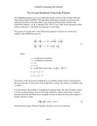
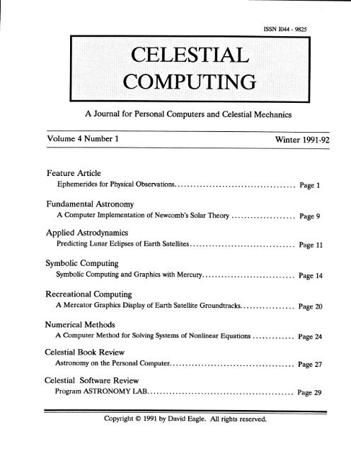
Vol.4 • No.. I Gele&iial GampuUnq, Wlnten 1991-92The format of the Mercury derivative function is DERIV(f (x) , x) where f(x) is theuser-defined function and x is the differentiation variable. In the GIOTA2equation file we first define the delta-V functions with the statementsdvtl(il) := vlc*sqrt(l+hl"2-2*hl*cos(il))+vlc*sqrt(h2"2*h3"2+h2"2-2*h2"2*h3*cos ( i t-i 1 ) )dvt2(i2) := Vlc*sqrt(l+hl"2-2*hl*cos(it-i2))+vlc*sqrt(h2"2*h3^2+h2"2-2*h2~2*h3*cos(i2))and then tell Mercury to differentiate them with the two statementsddvtdil = deriv(dvtHil), il)ddvtdi2 = deriv(dvt2(i2), 12)It is important to note that we can force Mercury to perform true symboliccomputing by not defining any of the other variables or constants of the problemwithin the equation file.The final results of the equation file are the two symbolic derivativesddvtdil= vlc*(-2*hl*(-SIN(il)))*0.5/SQRT(l+hl^2-2*hl*COS(il))ddvtdi2= vlc*(-2*hl*SIN(it-i2))*0.5/SQRT(l+hl^2-2*hl*COS(it-i2))+ vie* ( -2*h3* ( -SIN ( 12 ) ) *h2~2 ) *0. 5/SQRT (h2~2*h3"2+h2"2-2*h3*h2~2*COS ( 12 ) )The first derivative is the sensitivity of the total delta-V relative to thefirst plane change angle and the second equation is the partial derivative ofthe total delta-V with respect to the second plane change angle. Notice thatMercury does not attempt to simplify the final calculations.GIOTA3 is a third Mercury equation file which plots these two derivatives as afunction of plane change angle. This file was created by cutting and pastingthe derivative equations into the GIOTA1 equation file and changing the graphlabels and PLOT command. An examination of the graphics screen generated bythis file reveals that each plot crosses the Y = 0 axis at only one point.These are the two points at which the partial derivatives are zero. These twopoints are also the optimum plane change solutions of the orbit transferproblem. If you examine the original APPLIED ASTRODYNAMICS article, you willsee that this is exactly how the MathCAD equation file solved this problem.Again we have verified and visualized the results of numeric computation withcomputer graphics.Can you deduce the units of these two partial derivatives from the astrodynamicconstants and units used in the Mercury equation files?19

Vol. 4 • Na. I ^ele&LLat Computing, Wlnten 1991-92RECREATIONAL COMPUTINGGTRACK is a QuickBASIC computer program which will display the groundtrack of anEarth satellite on a Mercator map of the world. The groundtrack consists of thegeographic latitude and longitude of a satellite's subpoint at any instant. Thesubpoint is the point on the Earth's surface which is directly below a satellitein orbit. Program GTRACK plots groundtracks as a series of individual pixels tohelp you visualize the ground distance and direction travelled by any satelliteas a function of time. The software will also display North and South Americaon the Mercator projection. Support is provided for the CGA, EGA, VGA andHercules graphics modes of the IBM-PC and true compatible computers.The Y-coordinate of a Mercator projection is related to any geodetic latitude onthe map through the following equation:y = R In tan 45° + | (1)In this equation R is the circumference of the map, 0 is the geodetic latitude,and In is the natural logarithm. For a computer graphics display of a Mercatormap, the following relationships between the physical X and Y dimensions of thescreen and the Mercator equations exist:X and 0 = ± Jiv 360 ~"~ ^ "2The maximum and minimum latitudes which can be displayed on this type of map canbe determined by solving Eq. (1) for 0 as follows:0 = ± 2 tan^f eY/R I - 90" (2)Program GTRACK propagates satellite orbits using the method described in "FastOrbit Propagator for Graphical Display", by Landis Markley and James Jeletic,AIAA Journal of Guidance and Control, March-April 1991. This is a simple butefficient analytic orbit propagator which takes into account the differencebetween mean and osculating orbital elements. The algorithm is as follows:At the initial time a function which depends on the initial orbital elements ofthe satellite is defined by,. ^ ( 1 + e cos i>")3( . 0 . 2 . . 2 , , \)g(t ) = 1-3 sin i sin (v + w)0 v x __ e2 J IThis function is time dependent because the argument of perigee and true anomalychange as a function of time due to the perturbation caused by the oblate shapeof the Earth. This model assumes that the satellite's eccentricity e andorbital inclination i do not change.20

Vol.4 • Ma. 1 ^eleztlal Computing, Wlnten 1991-92The initial mean semimajor axis of a satellite is given bya = I a(to) + /a2(to) - 4J2R2g(to) | (4)and the corresponding mean mean motion is computed withn = fi± (5)v aThe mean semiparameter of the satellite is given byp = a (1 - e2) (6)The oblateness perturbations of the argument of perigee and east longitude ofthe ascending node are computed with the next two equations:( R 1 - fnI Pn J I2 - sin2i | (7)q ( p2 A\ - ^ J n cos i (8)2 2 I p JAt any time t the orbital elements are given byM = MQ + n (t - tQ) (9)A = AQ + A (t - t ) (10)w - w * w (t - tQ) (11)The osculating semimajor axis at time t is computed fromJ R2 g(t)a = a + - (12)awhere g(t) is Eq. (3) evaluated at this time with the updated orbital elementsGC>, and A.i>,The true anomaly required for this equation is found by solving Kepler'sequation using Newton's method and the current values of eccentricity and meananomaly. The Earth-centered-fixed (ECF) position vector of the satellite iscomputed with the standard orbital elements to state vector transformation. Thelatitude and longitude of the satellite's subpoint can be computed from theelements of the unit position vector as follows:21

Vol. 4 • No.. I Gele&tlal ^omputlru} Wlnten 1991-92 = sin'^R )A = ATAN3CR , R )x y(13a)(13b)ATAN3 in Eq. (13b) is a four quadrant inverse tangent function. The Mercatortransformation given by Eq.(1) is applied to the 0 calculation of Eq.(13a) andthen plotted by program GTRACK.Program NotesThe first thing the software will ask you for is the graphics mode of yourcomputer. Program GTRACK is set up to support the CGA, EGA, VGA and Herculesmode of the IBM-PC and true compatible computers. If you have QuickBASIC, it iseasy to change the SCREEN statements in the source code for other displays.The program will then ask you if you would like to perform a calibration of yourmonitor and graphics adapter. You should perform this procedure the first timeyou use the software and any time your graphics hardware changes. This processcustomizes the program for your system and determines how much of a Mercator mapcan be displayed. The program will draw both horizontal and vertical lines onyour screen and ask you to measure each. The units of measure can be inches orcentimeters or any convenient units. Please write down these measurements sothat you will not have to calibrate each time you use the software.You can specify both a latitude and longitude plot interval, in degrees, for theMercator display. These will help you visualize the location of the satellite'sgroundtrack on the Earth*s surface by displaying lines of constant latitude andlongitude on the map. If you input 0 for one or both of these requests, gridsof constant latitude/longitude will not be drawn.The program will then prompt you for an orbit propagation step size and thetotal number of orbits to plot. The step size must be input in minutes. Notethat it will take longer to propagate orbits with smaller step sizes.The final program requests are for the satellite's initial osculating orbitalelements. These elements include the satellite's perigee and apogee altitudes,orbital inclination, argument of perigee, and east longitude of the ascendingnode. Please note the proper units for each element and that east longitude canbe between 0 and 360 degrees.The program will also display North and South America on the graphics screen.The information required to do this is contained in the MAPLL.DAT data file onthe Celestial Computing floppy disk for this issue. This is an ASCII data fileof latitudes and corresponding longitudes for each geographic feature.The X-axis of the graphics map will be marked with both east and west longitudelabels. East longitude is measured to the right from 0 to 180 degrees and westlongitude is measured to the left, also from 0 to 180 degrees.22

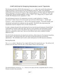
Vat. 4 • Na. 1 Gomputinq, Wlnten 1991-92The following is a typical Hercules screen display generated by program GTRACKfor two orbits of a repeating groundtrack Molniya satellite with the followinginitial osculating orbital elements:o perigee altitude = 663.4 kilometerso apogee altitude = 39,723.964 kilometerso orbital inclination = 63.435 degreeso argument of perigee = 270 degreeso east longitude of the ascending node = 0 degreesMercator Display of Satellite Groundtrack180 Longitude 188Figure 1Typical GTRACK Screen Display23

Vol. 4 • Ma. 1 Gele&tlat Gamputinq, Winten 1991-92NUMERICAL METHODSA general system of N nonlinear equations can be expressed in the form:V =(1)The solution of such a system of equations is the subject of this session ofNUMERICAL METHODS. NLBRENT.BAS is a QuickBASIC subroutine which can be used tosolve unconstrained systems of nonlinear equations using Brent*s method. Theterm unconstrained implies that there are no constraints on the values of thefinal solution vector X. The NLBRENT subroutine is a QuickBASIC implementationof the FORTRAN code described in the paper "BRENTM, A Fortran Subroutine for theNumerical Solution of Systems of Nonlinear Equations", by Jorge More and MichaelCosnard, ACM Transactions on Mathematical Software, Vol. 6, No. 2, June 1980.This is also ACM Algorithm 554.The following is description of subroutine NLBRENT. BAS and the proper proceduresfor calling and interacting with this software.SyntaxwhereCALL NLBRENT (N, X(), FVECO, TOL, MAXFEV, INFO, NFEV)N = number of equationsX() = input as the initial guess and output as the solution vectorTOL = convergence toleranceMAXFEV = maximum number of function evaluations allowedFVECO = residual vectorINFO = information flag1 = all residuals are at most TOL in magnitude2 = relative error between two successive iterates is at most TOL3 = conditions for both INFO = 1 and INFO = 2 hold4 = number of function evaluations >= MAXFEV5 = approximate Jacobian matrix is singular6 = iteration is not making good progress7 = iteration is diverging8 = iteration is converging, but TOL is too small, or the convergenceis very slow due to a Jacobian singular near the output X or dueto badly scaled variablesNFEV = number of actual function evaluations24

Vol. 4 • Na.l %ele&tial Gomputinq Wlnten 1991-92CommentsPlease note that the software uses the following type declarations:DEFINT I-NDEFDBL A-H, 0-ZThe system of nonlinear equations to be solved must be coded in a user-definedQuickBASIC subroutine with the following syntax:SUB USERFUNC (X(), FXO) STATICwhere X() is the current function argument vector and FX() is an array of one ormore function values evaluated at X().The companion disk for this issue includes a program called DEMONLE.BAS whichdemonstrates a typical application of subroutine NLBRENT. This demo programattempts to solve the system of nonlinear equations which define the conversionbetween geodetic and geocentric coordinates of a satellite.The mathematical relationship between geocentric and geodetic coordinatesgiven by the following system of two nonlinear equations:is(c + h) cos 0 - r cos 6=0 (2a)(s + h) sin 0 - r sin 6=0 (2b)wherer = geocentric distance6 = geocentric declinationh = geodetic altitude0 = geodetic latituderc =1 - (2f - f2) sin2s = c (1 - f)2r= equatorial radius of the Earth model (6378. 14 kilometers)f = flattening of the Earth model (1/298.257)A detailed description of this problem can be found in the SYMBOLIC COMPUTINGcolumn of the Volume 1, Number 2 (Spring 1989) issue of Celestial Computing.25

Vol. 4 • Na.l %ele&tial ^cmputinq, Winten 1991-92The following is the QuickBASIC source code listing of a user-defined subroutinewhich evaluates this system:SUB USERFUNC (X(), FXO) STATIC' Usei—defined system of non-linear equations subroutine' (C + ALTITUDE) # COS(LAT) - RMAG * COS(DECL) = 0' (S + ALTITUDE) * SIN(LAT) - RMAG * SIN(DECL) = 0* Input'X() = function argument vector' Output'END SUBFX() = array of function values evaluated at XXLAT = X(l)ALTITUDE = X(2)C = REQ / SQR(ltt - (2tt * FLAT - FLAT " 2) * SIN(XLAT) " 2)S = C # (Itt - FLAT) " 2FX(1) = (C + ALTITUDE) # COS(XLAT) - RMAG * COS(DECL)FX(2) = (S + ALTITUDE) * SIN(XLAT) - RMAG * SIN(DECL)The following is a typical output generated by DEMONLE. The program was given ageocentric declination of 45 degrees and a geocentric radius of 7500 kilometers.Program DEMONLE< Solution of a Non-linear System >Geodetic latitude (degrees) 45.16336606374469Geodetic altitude (kilometers) 1132.573865465997Value of residual tt 1Value of residual tt 2Number of iterations 8Convergence criteria .000000011.004050176334204D-10-3.836930773104541D-13The convergence criteria and the maximum number of iterations allowed arespecified by the user. The residuals are the errors between the solution foundby NLBRENT and the true value of zero for each equation of the nonlinear system.A geodetic latitude equal to the declination and a geodetic altitude equal tothe geocentric distance minus the polar radius of the Earth were used as initialguesses for this example.26

Vol. 4 • No.. I Geie&tiat gomputtag Winter 1991-92CELESTIAL BOOK REVIEWAstronomy on the Personal Computer by Oliver Montenbruck and Thomas Pfleger,Springer-Verlag, 1991. $50 hardbound with 5 1/4" companion floppy disk for theIBM-PC and true compatible computers.Astronomy on the Personal Computer successfully combines technical informationand practical software in a refreshing, innovative way. Each chapter containsinformation and equations which describe a particular astronomical problem alongwith an excellent companion computer program. Within the pages of Astronomy onthe Personal Computer we find numerical treatment of such items as Chebyshevseries representation of ephemerides, a clever way to predict the times ofgeocentric conjunction, and a complete photographic reduction program.The following is a compilation and brief description of the main chapter topics:o Coordinate Systems - this chapter discusses fundamental astronomicalconcepts such as Calendar and Julian Dates, ecliptic and equatorialcoordinates, precession, geocentric coordinates and the Sun's orbit.o Calculation of Rising and Setting Times - this chapter demonstrates howto use quadratic interpolation to determine rising and setting times ofthe Sun and Moon.o Cometary Orbits - this chapter discusses how to compute ephemerides ofcomets and minor planets. It also includes a method for near-parabolicorbits using Stumpff functions.o Planetary Orbits - this chapter demonstrates how to compute the positionsof the Sun and planets for a given date.o The Orbit of the Moon - this chapter shows how to use Chebyshev series tocompute a lunar ephemeris based on Brown* s theory.o Solar Eclipses - this chapter provides a way to compute the coordinatesof the central line of a solar eclipse. It also includes a neat methodfor calculating the times of a New Moon.o Stellar Occultations - this chapter shows how to construct software whichcan predict lunar occultations of stellar objects.o Orbit Determination - this chapter addresses the problem of determiningthe orbit of a comet or minor planet using Gauss's method and threegeocentric observations.o Astrometry - the material in this chapter shows how to determine thepositions of celestial objects from photographs of the sky.27

Vol.4 • No.. I ^eletitial ^omputiruq, Wlnten 1991-92Each chapter contains commented source code listings and a numerical example forthe main program. The code comments include a description of each and everyinput and output used in a procedure as well as the proper units. Many of theapplications are "data-driven" using small input data files which you can createand modify with an editor or Turbo Pascal. The proper format of each and everydata file is carefully explained. A "Notes on Alterations to Suit IndividualComputers" appendix is included which will help those who might want to port thesoftware to other computers and implementations of PASCAL.PASCAL source code listings of procedure, functions and driver programs areprovided in a modular and easy to understand fashion. PASCAL has always beenone of my favorite languages because it contains so many useful constructs anddoes not allow the user to write sloppy code. My only complaint about thesoftware is that executable code is not included on the companion floppy disk.To actually use the software, you will have to purchase some version of PASCALand compile and link the source code. Although the book talks about generallanguage requirements, the software is easiest to use with Borland's TurboPascal. The README file states that the programs should work with Turbo Pascalversion 4.0 and later. I used Turbo Pascal 6.0 which can be purchased by mailorder for about $100. A Windows version of Turbo Pascal is also available.Once the proper PATH statements were in place, the compilations were easy andautomatic from within the Turbo Pascal environment.The software is organized on the disk as main program files, input data files,units definition files and procedures and functions. Everything is very modularand it would be easy to build your own PASCAL applications using this toolbox.The following is a short list of the software ingredients:o Main Programso Input Datao Units Definition Fileso Subroutines for Calculating Keplerian Orbitso Mathematical Subroutineso Lunar Orbito Planetary Positionso Precession and Nutationo Spherical Astronomyo Solar Orbito Time and Calendaro DiverseI really like both Astronomy with the Personal Computer and its companionsoftware. I can recommend it to anyone who wants to learn how to reduce complexastronomical concepts to practical computer programs.28

Vol. 4 • Na. 1 Geleotial Gamputlnq. Wlnten 1991-92CELESTIAL SOFTWARE REVIEWAstronomy Lab, Personal MicroCosms, 8547 E. Arapahoe Road, Suite J-147,Greenwood Village, CO 80112, (303) 753-3268. Available for the IBM-PC and truecompatible computers, 3 1/2" and 5 1/4" disk formats. Price: US & Canada $59.95+ $2.95 first-class, Overseas US $59.95 + $14.95 airmail.Astronomy Lab is a versatile computer program which combines astronomicalanimation, computer graphics and numerical data in a unique way for the IBM-PCand true compatible computers. Astronomy Lab can produce color movies thatsimulate a variety of astronomical phenomena, graphical charts that illustratemany fundamental concepts of astronomy, and printed reports that providepredictions of important astronomical events. All movies, charts, and reportscan be customized for the user's geographic location and time zone. AstronomyLab is one of the few astronomy programs I have seen which actually teaches theuser about basic astronomy using color computer graphics.Astronomy Lab requires at least 512K of memory, MS-DOS 3.0 or later, a hard diskor high-density floppy disk drive, and EGA or VGA graphics. A PC with an 80286or above CPU is recommended. I have been informed by the author of AstronomyLab, Eric Bergman-Terrell, that a version is also available for Windows. Thereview described here is for the DOS version of the software. This versioncomes with both a coprocessor and non-coprocessor version of the main program.As with any computation intensive software, a coprocessor is highly recommended!Astronomy Lab will also support Epson and Postscript compatible printers. Amouse is not required or supported in the DOS version.The software uses pull-down menus with dialog boxes and is quite intuitive. Itis easy to toggle different selections of which there are many. The 153 pageuser's manual is well written and comprehensive. This manual contains atutorial introduction to the software, a chapter on exploring astronomy usingAstronomy Lab, and an activities section. The items in the activities chapterare quite clever and easily demonstrate how to use Astronomy Lab to learn andexplore. Chapter 5 talks about how to use Astronomy Lab with spreadsheetsoftware and there are many helpful illustrations throughout. This chapterdemonstrates how to graph the information produced by the data produced byAstronomy Lab reports. The manual appendices contain a variety of supplementalinformation such as the following:o Basic Astronomical Conceptso Recommended Readingo Answers to Numbered Questionso Location Information for U.S., Canadian, and World Citieso Using a Math Coprocessor29

Vol. 4 • Na.l %e&e&tiat gomputmg Wlnten 1991-92The following is a brief description of the main Astronomy Lab features.MoviesAstronomy Lab movies can be used to simulate and visualize a variety ofastronomical phenomena. Each frame of a movie can be printed to an Epson orPostscript compatible printer. The type of movies which can be generated areChartso Night Sky - a movie of the night sky with the sun, moon and planetso Day/Night - a movie of the sunlit regions of the Eartho Ecliptic 1 - planet orbits as viewed from above the ecliptico Ecliptic 2 - a side view of the planetary orbitso Jupiter Moons 1 - orbits of Jupiter's moons as viewed from Eartho Jupiter Moon 2 - orbits of Jupiter's moons as viewed from above JupiterThe charts displayed by Astronomy Lab are graphs of important astronomicalinformation. Some of the graphs which can be generated areReportso Planet Orbits - a graph of right ascension as a function of timeo Jupiter Moons Orbit - configurations of Jupiter's moonso Planet Magnitude, Illumination Fraction, Diameter and Distanceo Equation of Time - a graph of the equation of time for one yearo Day length - a graph of the length of days for one yearAstronomy Lab reports generate numerical data about' astronomical events. Thesereports can be viewed on the screen, printed on a printer, or saved to a diskfile. A partial list of the types of reports which the user can calculate areo Calendar - a yearly calendar of sunrise, sunset, moonrise, moonset, solarand lunar eclipses, lunar phases, equinoxes and solstices.o Solar Eclipses - circumstances of solar eclipseso Seasons - equinoxes, solstices and lengths of seasonso Dates of Easter - calendar dates of Eastero Lunar Eclipses - circumstances of lunar eclipseso Planet View, Apsides, Conjunctions, Oppositions, Datao Moon Apsides - dates of lunar apogee and perigeeo Almanac - generates all reports at once30

Vol. 4 • Na. 1 Computing, Wlnten 1991-92DISK INFORMATIONThe CELESTIAL COMPUTING floppy disk contains QuickBASIC source code, executablefiles, and the Mercury source and report files for the articles presented inthis issue. The disk also contains a latitude/longitude database file.The following is a directory listing of the files on the disk for this issue.BRUN45DEMONLEDEMONLEGIOTA1GIOTA2GIOTA2GIOTA3GTRACKGTRACKEXEBASEXEEKAEKARPTEKABASEXE774401268212208245989618772203123301306709-28-8812-15-9112-15-9110-05-9110-14-9110-14-9112-18-9110-07-9110-07-91LESATLESATMAPLLNLBRENTPEPHEMPEPHEMQBHERCSOLARSOLARBASEXEDATBASBASEXECOMBASEXE287002710228258701638325406366947162001912010-23-9110-23-9110-04-9109-25-9112-24-9112-24-9103-06-9110-03-9110-03-91The QuickBASIC source files have the DOS filename extension *.BAS and executablefiles all end in *.EXE. Each executable program requires the QuickBASICBRUN45.EXE file to work properly. The Mercury equation files have a *.EKAfilename and the companion report files end with *.RPT. Each equation file canbe loaded into Mercury with the command, Mercury filename, eka. Mercury reportfiles can be examined with an editor. Executable files can be run by simplytyping their name at the DOS prompt. Source files can be brought into theQuickBASIC environment by typing QB filename. The latitude and longitudedatabase file is named MAPLL.DAT.MAPLL.DAT is a "pure" ASCII data file which contains integer indices and pairsof latitude and longitude coordinates. The number of coordinate pairs for eachgeographic feature is specified by the indices. The numerical coordinates arein the units of radians where latitude ranges between ± n/2 and longitude ismeasured positive east of Greenwich and ranges between 0 and 2n radians. Thefirst and last coordinate pairs are identical so that a graphics representationwill close upon itself.The floppy disk also contains the following files.> BRUN45.EXE - this is the run-time program required for all QuickBASICexecutable programs. When copying Celestial Computing QuickBASICexecutable programs to other floppy and hard disks, be sure to copy thisfile also.o QBHERC. COM - this file is required when using Hercules compatiblegraphics boards with QuickBASIC programs which display graphics. Thisprogram must be run before executing any graphics program. It can beinvoked from the DOS command line by typing QBHERC.31

Vol. 4 • Na. 1 Wlnten 1991-92SUBSCRIPTION AND DISK INFORMATIONCelestial Computing is published four times per year, around the time of thesolstices and equinoxes (March, June, September and December). Both journal andfloppy disk subscriptions for the IBM-PC and compatibles are available. Thewritten journal contains a technical discussion about each article andinstructions which explain how to use the software. The floppy disk containsthe actual computer programs.The computer programs are available on both 5 1/4", 360K capacity floppy disksand 3 1/2", 720K capacity floppy disks. Please be sure to specify the formatwhen ordering disk subscriptions. Both QuickBASIC source code and executableprograms are provided on the disks. The Microsoft QuickBASIC compiler is notrequired to run these programs.Please submit payment in the form of a personal check or money order (no creditcards please), in U.S. dollars and drawn on a U.S. bank, payable to ScienceSoftware. The costs to countries other than the United States are shown inparentheses. These prices include first class shipping within the United Statesand air mail shipping elsewhere. Please send all orders and correspondence to:Science Software7370 S. Jay StreetLittleton, CO 80123-4661Celestial Computing Subscription FormnnnCelestial Computing journal subscription( 1 year, 4 issues ) $29.95 ($39.95)Celestial Computing disk subscription( 1 year, 4 disks ) $19.95 ($24.95)Celestial Computing back issueso journal $7.95 ($9.95) o disk $5.95 ($6.95)indicate issue(s) by volume and numberPlease specify the disk formatD 5 1/4", 360K n 3 1/2", 720KNameStreet addressCity, state, zip32

Vol. 4 • Nci.l Gele&tiat Gamputinq. Wint&i 1991-92COMING NEXT ISSUEo Feature ArticleA Computer Implementation of the Brouwer-Lyddane Orbit Theoryo Fundamental AstronomyPredicting Rise, Transit and Set of Celestial Objectso Applied AstrodynamicsConverting Between Osculating and Mean Orbital Elementso Symbolic ComputingDesigning Repeating Groundtrack Orbits with Mercuryo Recreational ComputingComputer Graphic Displays of the Earth From Spaceo Numerical MethodsEvaluating the ICE Chebyshev CoefficientsERRATUMThe last sentence of the second paragraph on page 14 of the Spring 1991 issueshould be:Furthermore, the software eliminates the logic required to determine whenrectification should occur by simply rectifying the orbit after each and everypropagation step.IBM is a registered trademark of the IBM Corporation.QuickBASIC, MS-DOS and Windows are registered trademarks of Microsoft Corp.Mercury is copyright © 1990 by Roger Schlafly.Hercules is a registered trademark of Hercules Computer Technology.MathCAD is a registered trademark of MathSoft, Inc.Turbo Pascal is a registered trademark of Borland International.33

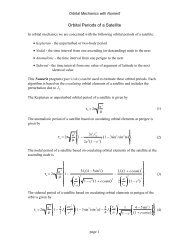
1P\1 T 7 T 7 T 1" ill"lo ITo \1in*/o iini oil/r^iniUPItdl V Vb> IIlCIiliciLIUIidvt!(ACLdvt2dv1dv2LJQ0.000.0 10. 20. 30.INCLINATION (deg)

Sensitivitessiveddvtdi!0.50ddvtdi2o-0.50-1.00.0 10. 20. 30.INCLINATION