University of California - Leif and Vera Svalgaard's

More documents

Recommendations

Info

Falls Creek Proposed Hydroelectric ProjectReconnaissance Reportstream gradient is 418 ftlmi and stream width averages 15 ft wide. The Falls Creek substrateincludes cobble, boulder deposits, few gravel bars and a thin layer of fine silt near the mouth; thelower one mile of stream has been extensively channelized and modified by placer mining (APA1984). Three to four acres adjacent to the active channel in the lower 0.5 miles are covered withtailings and 100 yards of the streambed in this area has been relocated (AEIDC 1982).The lower 2,300 ft of Falls Creek is classified as anadromous in the ADF&G AnadromousWaters Catalog (A WC). Anadromous fish species present in Falls Creek included juvenileChinook (Oncorhynchus tshawytscha) and juvenile Dolly Varden (Salve linus malma) (USFWS1961, Johnson and Daigneault 2008, AEIDC 1982).Previous StudiesThe hydroelectric potential at Grant Lake, approximately 1 mile north of Falls Creek, has beenevaluated several times as a potential power source for the SewardlKenai Peninsula area. In1954 R.W. Beck and Associates (cited in APA 1984) prepared a preliminary investigation andconcluded that a project was feasible. In 1980 CH2M Hill (cited in APA 1984) prepared a prefeasibilitystudy for a Grant Lake project and concluded that a project developed at the site wasfeasible.The most extensive study was performed by Ebasco Services, Inc. in 1984 for the Alaska PowerAuthority (APA 1984). Falls Creek (Figure 1) was investigated by Ebasco in 1984 for theAlaska Power Authority (now Alaska Energy Authority) as a possible source of additional flowsthat could be diverted to nearby Grant Lake in support of a hydroelectric project there (APA1984).Environmental ConsiderationsThe following presents a general overview of potential expected environmental considerationsfor a hydroelectric project at Falls Creek. This section describes fish resources, wetlands,hydrology and water quality, recreation, subsistence, and cultural resources of the project area.The area is managed using several specific management plans, including the Chugach NationalForest Plan (Meade 2006), Kenai River Comprehensive Management Plan (DNR 1998), andKenai Borough Coastal Management Plan (KPB 2008). Another search for all relevant landmanagement plans would be required as part of FERC licensing and by other required permittingprocesses.Ebasco (APA 1984) compiled a feasibility report on the Grant Lake hydroelectric project,including detailed environmental studies of water use and quality; aquatic, botanical and wildliferesources; historical and archaeological resources; socioeconomic impacts; geological and soilresources; recreational resources; aesthetic resources; and land use. The Arctic EnvironmentalData Center (AIEDC 1982 and 1983) and USFWS (1961) conducted environmental baselinestudies in the project area. For the purposes of this feasibility report, HDR Alaska did notconduct any environmental work beyond initial reconnaissance visits and instantaneous flowmeasurements (see Hydrology and Water Quality below) and this overview draws mainly onthese historical reports.2
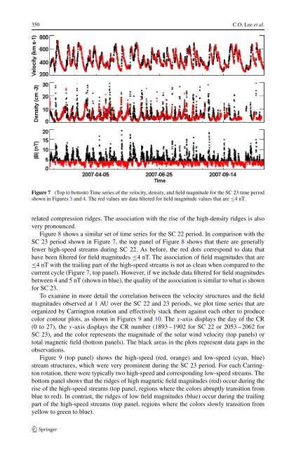
350 C.O. Lee et al.Figure 7 (Top to bottom) Time series of the velocity, density, and field magnitude for the SC 23 time periodshown in Figures 3 and 4. The red values are data filtered for field magnitude values that are ≤4nT.related compression ridges. The association with the rise of the high-density ridges is alsovery pronounced.Figure 8 shows a similar set of time series for the SC 22 period. In comparison with theSC 23 period shown in Figure 7, the top panel of Figure 8 shows that there are generallyfewer high-speed streams during SC 22. As before, the red dots correspond to data thathave been filtered for field magnitudes ≤4 nT. The association of field magnitudes that are≤4 nT with the trailing part of the high-speed streams is not as clean when compared to thecurrent cycle (Figure 7, top panel). However, if we include data filtered for field magnitudesbetween 4 and 5 nT (shown in blue), the quality of the association is similar to what is shownfor SC 23.To examine in more detail the correlation between the velocity structures and the fieldmagnitudes observed at 1 AU over the SC 22 and 23 periods, we plot time series that areorganized by Carrington rotation and effectively stack them against each other to producecolor contour plots, as shown in Figures 9 and 10. Thex-axis displays the day of the CR(0 to 27), the y-axis displays the CR number (1893 – 1902 for SC 22 or 2053 – 2062 forSC 23), and the color represents the magnitude of the solar wind velocity (top panels) ortotal magnetic field (bottom panels). The black areas in the plots represent data gaps in theobservations.Figure 9 (top panel) shows the high-speed (red, orange) and low-speed (cyan, blue)stream structures, which were very prominent during the SC 23 period. For each Carringtonrotation, there were typically two high-speed and corresponding low-speed streams. Thebottom panel shows that the ridges of high magnetic field magnitudes (red) occur during therise of the high-speed streams (top panel, regions where the colors abruptly transition fromblue to red). In contrast, the ridges of low field magnitudes (blue) occur during the trailingpart of the high-speed streams (top panel, regions where the colors slowly transition fromyellow to green to blue).
Page 1: University of CaliforniaPeer Review
Page 5: 348 C.O. Lee et al.Figure 3 Histogr
Page 9 and 10: 352 C.O. Lee et al.Figure 10 Color
Page 11 and 12: 354 C.O. Lee et al.Figure 12 The de
Page 13 and 14: 356 C.O. Lee et al.Figure 14 Global
Page 15 and 16: 358 C.O. Lee et al.Figure 15 Global
Page 17 and 18: 360 C.O. Lee et al.Figure 17 Numeri
Page 19 and 20: 362 C.O. Lee et al.SC 23 period, th

University of California - Leif and Vera Svalgaard's

You also want an ePaper? Increase the reach of your titles

Delete template?

Save as template?