1 Introduction

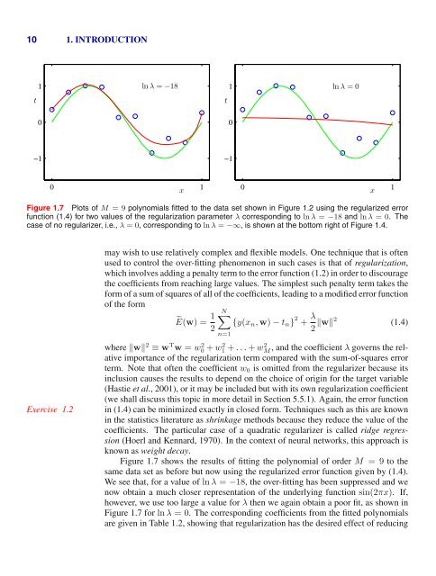
10 1. INTRODUCTION1ln λ = −181ln λ =0tt00−1−10x10x1Figure 1.7 Plots of M =9polynomials fitted to the data set shown in Figure 1.2 using the regularized errorfunction (1.4) for two values of the regularization parameter λ corresponding to ln λ = −18 and ln λ =0. Thecase of no regularizer, i.e., λ =0, corresponding to ln λ = −∞, is shown at the bottom right of Figure 1.4.Exercise 1.2may wish to use relatively complex and flexible models. One technique that is oftenused to control the over-fitting phenomenon in such cases is that of regularization,which involves adding a penalty term to the error function (1.2) in order to discouragethe coefficients from reaching large values. The simplest such penalty term takes theform of a sum of squares of all of the coefficients, leading to a modified error functionof the formẼ(w) = 1 N∑{y(x n , w) − t n } 2 + λ 22 ‖w‖2 (1.4)n=1where ‖w‖ 2 ≡ w T w = w0 2 + w1 2 + ...+ wM 2 , and the coefficient λ governs the relativeimportance of the regularization term compared with the sum-of-squares errorterm. Note that often the coefficient w 0 is omitted from the regularizer because itsinclusion causes the results to depend on the choice of origin for the target variable(Hastie et al., 2001), or it may be included but with its own regularization coefficient(we shall discuss this topic in more detail in Section 5.5.1). Again, the error functionin (1.4) can be minimized exactly in closed form. Techniques such as this are knownin the statistics literature as shrinkage methods because they reduce the value of thecoefficients. The particular case of a quadratic regularizer is called ridge regression(Hoerl and Kennard, 1970). In the context of neural networks, this approach isknown as weight decay.Figure 1.7 shows the results of fitting the polynomial of order M =9to thesame data set as before but now using the regularized error function given by (1.4).We see that, for a value of ln λ = −18, the over-fitting has been suppressed and wenow obtain a much closer representation of the underlying function sin(2πx). If,however, we use too large a value for λ then we again obtain a poor fit, as shown inFigure 1.7 for ln λ =0. The corresponding coefficients from the fitted polynomialsare given in Table 1.2, showing that regularization has the desired effect of reducing