1 Introduction

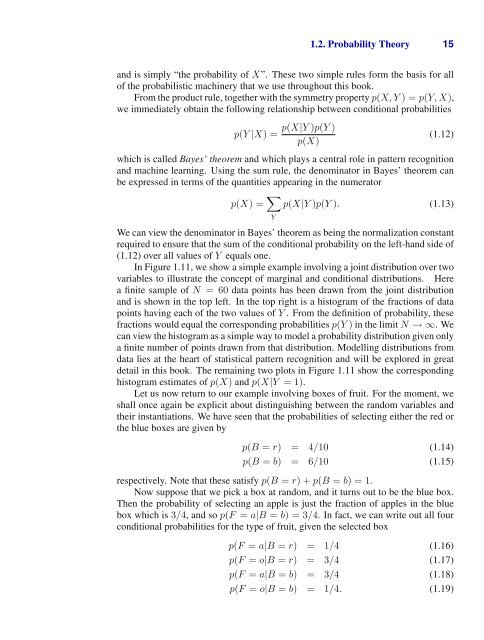
1.2. Probability Theory 15and is simply “the probability of X”. These two simple rules form the basis for allof the probabilistic machinery that we use throughout this book.From the product rule, together with the symmetry property p(X, Y )=p(Y,X),we immediately obtain the following relationship between conditional probabilitiesp(X|Y )p(Y )p(Y |X) = (1.12)p(X)which is called Bayes’ theorem and which plays a central role in pattern recognitionand machine learning. Using the sum rule, the denominator in Bayes’ theorem canbe expressed in terms of the quantities appearing in the numeratorp(X) = ∑ Yp(X|Y )p(Y ). (1.13)We can view the denominator in Bayes’ theorem as being the normalization constantrequired to ensure that the sum of the conditional probability on the left-hand side of(1.12) over all values of Y equals one.In Figure 1.11, we show a simple example involving a joint distribution over twovariables to illustrate the concept of marginal and conditional distributions. Herea finite sample of N =60data points has been drawn from the joint distributionand is shown in the top left. In the top right is a histogram of the fractions of datapoints having each of the two values of Y . From the definition of probability, thesefractions would equal the corresponding probabilities p(Y ) in the limit N →∞.Wecan view the histogram as a simple way to model a probability distribution given onlya finite number of points drawn from that distribution. Modelling distributions fromdata lies at the heart of statistical pattern recognition and will be explored in greatdetail in this book. The remaining two plots in Figure 1.11 show the correspondinghistogram estimates of p(X) and p(X|Y =1).Let us now return to our example involving boxes of fruit. For the moment, weshall once again be explicit about distinguishing between the random variables andtheir instantiations. We have seen that the probabilities of selecting either the red orthe blue boxes are given byp(B = r) = 4/10 (1.14)p(B = b) = 6/10 (1.15)respectively. Note that these satisfy p(B = r)+p(B = b) =1.Now suppose that we pick a box at random, and it turns out to be the blue box.Then the probability of selecting an apple is just the fraction of apples in the bluebox which is 3/4, and so p(F = a|B = b) =3/4. In fact, we can write out all fourconditional probabilities for the type of fruit, given the selected boxp(F = a|B = r) = 1/4 (1.16)p(F = o|B = r) = 3/4 (1.17)p(F = a|B = b) = 3/4 (1.18)p(F = o|B = b) = 1/4. (1.19)