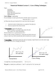
26 1. INTRODUCTIONFigure 1.14Illustration of the likelihood function fora Gaussian distribution, shown by thered curve. Here the black points denotea data set of values {x n}, andthe likelihood function given by (1.53)corresponds to the product of the bluevalues. Maximizing the likelihood involvesadjusting the mean and varianceof the Gaussian so as to maximizethis product.p(x)x nN (x n |µ, σ 2 )xNow suppose that we have a data set of observations x =(x 1 ,...,x N ) T , representingN observations of the scalar variable x. Note that we are using the typefacex to distinguish this from a single observation of the vector-valued variable(x 1 ,...,x D ) T , which we denote by x. We shall suppose that the observations aredrawn independently from a Gaussian distribution whose mean µ and variance σ 2are unknown, and we would like to determine these parameters from the data set.Data points that are drawn independently from the same distribution are said to beindependent and identically distributed, which is often abbreviated to i.i.d. We haveseen that the joint probability of two independent events is given by the product ofthe marginal probabilities for each event separately. Because our data set x is i.i.d.,we can therefore write the probability of the data set, given µ and σ 2 , in the formp(x|µ, σ 2 )=N∏N ( x n |µ, σ 2) . (1.53)n=1Section 1.2.5When viewed as a function of µ and σ 2 , this is the likelihood function for the Gaussianand is interpreted diagrammatically in Figure 1.14.One common criterion for determining the parameters in a probability distributionusing an observed data set is to find the parameter values that maximize thelikelihood function. This might seem like a strange criterion because, from our foregoingdiscussion of probability theory, it would seem more natural to maximize theprobability of the parameters given the data, not the probability of the data given theparameters. In fact, these two criteria are related, as we shall discuss in the contextof curve fitting.For the moment, however, we shall determine values for the unknown parametersµ and σ 2 in the Gaussian by maximizing the likelihood function (1.53). In practice,it is more convenient to maximize the log of the likelihood function. Becausethe logarithm is a monotonically increasing function of its argument, maximizationof the log of a function is equivalent to maximization of the function itself. Takingthe log not only simplifies the subsequent mathematical analysis, but it also helpsnumerically because the product of a large number of small probabilities can easilyunderflow the numerical precision of the computer, and this is resolved by computinginstead the sum of the log probabilities. From (1.46) and (1.53), the log likelihood
1.2. Probability Theory 27function can be written in the formExercise 1.11Section 1.1Exercise 1.12ln p ( x|µ, σ 2) = − 12σ 2N∑n=1(x n − µ) 2 − N 2 ln σ2 − N 2ln(2π). (1.54)Maximizing (1.54) with respect to µ, we obtain the maximum likelihood solutiongiven byµ ML = 1 N∑x n (1.55)Nwhich is the sample mean, i.e., the mean of the observed values {x n }. Similarly,maximizing (1.54) with respect to σ 2 , we obtain the maximum likelihood solutionfor the variance in the formσ 2 ML = 1 Nn=1N∑(x n − µ ML ) 2 (1.56)n=1which is the sample variance measured with respect to the sample mean µ ML . Notethat we are performing a joint maximization of (1.54) with respect to µ and σ 2 ,butin the case of the Gaussian distribution the solution for µ decouples from that for σ 2so that we can first evaluate (1.55) and then subsequently use this result to evaluate(1.56).Later in this chapter, and also in subsequent chapters, we shall highlight the significantlimitations of the maximum likelihood approach. Here we give an indicationof the problem in the context of our solutions for the maximum likelihood parametersettings for the univariate Gaussian distribution. In particular, we shall showthat the maximum likelihood approach systematically underestimates the varianceof the distribution. This is an example of a phenomenon called bias and is relatedto the problem of over-fitting encountered in the context of polynomial curve fitting.We first note that the maximum likelihood solutions µ ML and σML 2 are functions ofthe data set values x 1 ,...,x N . Consider the expectations of these quantities withrespect to the data set values, which themselves come from a Gaussian distributionwith parameters µ and σ 2 . It is straightforward to show thatE[µ ML ] = µ (1.57)( ) N − 1E[σML] 2 =σ 2 (1.58)Nso that on average the maximum likelihood estimate will obtain the correct mean butwill underestimate the true variance by a factor (N − 1)/N . The intuition behindthis result is given by Figure 1.15.From (1.58) it follows that the following estimate for the variance parameter isunbiased˜σ 2 =NN − 1 σ2 ML = 1 N∑(x n − µ ML ) 2 . (1.59)N − 1n=1