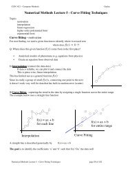
24 1. INTRODUCTIONsee, is required in order to make predictions or to compare different models. Thedevelopment of sampling methods, such as Markov chain Monte Carlo (discussed inChapter 11) along with dramatic improvements in the speed and memory capacityof computers, opened the door to the practical use of Bayesian techniques in an impressiverange of problem domains. Monte Carlo methods are very flexible and canbe applied to a wide range of models. However, they are computationally intensiveand have mainly been used for small-scale problems.More recently, highly efficient deterministic approximation schemes such asvariational Bayes and expectation propagation (discussed in Chapter 10) have beendeveloped. These offer a complementary alternative to sampling methods and haveallowed Bayesian techniques to be used in large-scale applications (Blei et al., 2003).1.2.4 The Gaussian distributionWe shall devote the whole of Chapter 2 to a study of various probability distributionsand their key properties. It is convenient, however, to introduce here oneof the most important probability distributions for continuous variables, called thenormal or Gaussian distribution. We shall make extensive use of this distribution inthe remainder of this chapter and indeed throughout much of the book.For the case of a single real-valued variable x, the Gaussian distribution is definedbyN ( {x|µ, σ 2) 1=(2πσ 2 ) exp − 1 }1/2 2σ (x − 2 µ)2 (1.46)which is governed by two parameters: µ, called the mean, and σ 2 , called the variance.The square root of the variance, given by σ, is called the standard deviation,and the reciprocal of the variance, written as β =1/σ 2 , is called the precision. Weshall see the motivation for these terms shortly. Figure 1.13 shows a plot of theGaussian distribution.From the form of (1.46) we see that the Gaussian distribution satisfiesN (x|µ, σ 2 ) > 0. (1.47)Exercise 1.7Also it is straightforward to show that the Gaussian is normalized, so thatPierre-Simon Laplace1749–1827It is said that Laplace was seriouslylacking in modesty and at onepoint declared himself to be thebest mathematician in France at thetime, a claim that was arguably true.As well as being prolific in mathematics,he also made numerous contributions to astronomy,including the nebular hypothesis by which theearth is thought to have formed from the condensationand cooling of a large rotating disk of gas anddust. In 1812 he published the first edition of ThéorieAnalytique des Probabilités, in which Laplace statesthat “probability theory is nothing but common sensereduced to calculation”. This work included a discussionof the inverse probability calculation (later termedBayes’ theorem by Poincaré), which he used to solveproblems in life expectancy, jurisprudence, planetarymasses, triangulation, and error estimation.
1.2. Probability Theory 25Figure 1.13Plot of the univariate Gaussianshowing the mean µ and thestandard deviation σ.N (x|µ, σ 2 )2σµxExercise 1.8∫ ∞−∞N ( x|µ, σ 2) dx =1. (1.48)Thus (1.46) satisfies the two requirements for a valid probability density.We can readily find expectations of functions of x under the Gaussian distribution.In particular, the average value of x is given byE[x] =∫ ∞−∞N ( x|µ, σ 2) x dx = µ. (1.49)Because the parameter µ represents the average value of x under the distribution, itis referred to as the mean. Similarly, for the second order moment∫ ∞E[x 2 ]= N ( x|µ, σ 2) x 2 dx = µ 2 + σ 2 . (1.50)−∞From (1.49) and (1.50), it follows that the variance of x is given byvar[x] =E[x 2 ] − E[x] 2 = σ 2 (1.51)Exercise 1.9and hence σ 2 is referred to as the variance parameter. The maximum of a distributionis known as its mode. For a Gaussian, the mode coincides with the mean.We are also interested in the Gaussian distribution defined over a D-dimensionalvector x of continuous variables, which is given by{1 1N (x|µ, Σ) =(2π) D/2 |Σ| exp − 1 }1/2 2 (x − µ)T Σ −1 (x − µ) (1.52)where the D-dimensional vector µ is called the mean, the D × D matrix Σ is calledthe covariance, and |Σ| denotes the determinant of Σ. We shall make use of themultivariate Gaussian distribution briefly in this chapter, although its properties willbe studied in detail in Section 2.3.