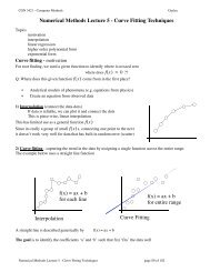
36 1. INTRODUCTIONextend this approach to deal with input spaces having several variables. If we haveD input variables, then a general polynomial with coefficients up to order 3 wouldtake the formy(x, w) =w 0 +D∑w i x i +i=1D∑i=1 j=1D∑w ij x i x j +D∑D∑i=1 j=1 k=1D∑w ijk x i x j x k . (1.74)Exercise 1.16As D increases, so the number of independent coefficients (not all of the coefficientsare independent due to interchange symmetries amongst the x variables) grows proportionallyto D 3 . In practice, to capture complex dependencies in the data, we mayneed to use a higher-order polynomial. For a polynomial of order M, the growth inthe number of coefficients is like D M . Although this is now a power law growth,rather than an exponential growth, it still points to the method becoming rapidlyunwieldy and of limited practical utility.Our geometrical intuitions, formed through a life spent in a space of three dimensions,can fail badly when we consider spaces of higher dimensionality. As asimple example, consider a sphere of radius r =1in a space of D dimensions, andask what is the fraction of the volume of the sphere that lies between radius r =1−ɛand r =1. We can evaluate this fraction by noting that the volume of a sphere ofradius r in D dimensions must scale as r D , and so we writeV D (r) =K D r D (1.75)Exercise 1.18where the constant K D depends only on D. Thus the required fraction is given byV D (1) − V D (1 − ɛ)V D (1)=1− (1 − ɛ) D (1.76)Exercise 1.20which is plotted as a function of ɛ for various values of D in Figure 1.22. We seethat, for large D, this fraction tends to 1 even for small values of ɛ. Thus, in spacesof high dimensionality, most of the volume of a sphere is concentrated in a thin shellnear the surface!As a further example, of direct relevance to pattern recognition, consider thebehaviour of a Gaussian distribution in a high-dimensional space. If we transformfrom Cartesian to polar coordinates, and then integrate out the directional variables,we obtain an expression for the density p(r) as a function of radius r from the origin.Thus p(r)δr is the probability mass inside a thin shell of thickness δr located atradius r. This distribution is plotted, for various values of D, in Figure 1.23, and wesee that for large D the probability mass of the Gaussian is concentrated in a thinshell.The severe difficulty that can arise in spaces of many dimensions is sometimescalled the curse of dimensionality (Bellman, 1961). In this book, we shall make extensiveuse of illustrative examples involving input spaces of one or two dimensions,because this makes it particularly easy to illustrate the techniques graphically. Thereader should be warned, however, that not all intuitions developed in spaces of lowdimensionality will generalize to spaces of many dimensions.
1.4. The Curse of Dimensionality 37Figure 1.22Plot of the fraction of the volume ofa sphere lying in the range r =1−ɛto r = 1 for various values of thedimensionality D.10.8D =20D =5volume fraction0.60.4D =2D =10.200 0.2 0.4 0.6 0.8 1ɛAlthough the curse of dimensionality certainly raises important issues for patternrecognition applications, it does not prevent us from finding effective techniquesapplicable to high-dimensional spaces. The reasons for this are twofold. First, realdata will often be confined to a region of the space having lower effective dimensionality,and in particular the directions over which important variations in the targetvariables occur may be so confined. Second, real data will typically exhibit somesmoothness properties (at least locally) so that for the most part small changes in theinput variables will produce small changes in the target variables, and so we can exploitlocal interpolation-like techniques to allow us to make predictions of the targetvariables for new values of the input variables. Successful pattern recognition techniquesexploit one or both of these properties. Consider, for example, an applicationin manufacturing in which images are captured of identical planar objects on a conveyorbelt, in which the goal is to determine their orientation. Each image is a pointFigure 1.23Plot of the probability density withrespect to radius r of a Gaussiandistribution for various valuesof the dimensionality D. In ahigh-dimensional space, most of theprobability mass of a Gaussian is locatedwithin a thin shell at a specificradius.p(r)21D =1D =2D =2000 2 4r