1 Introduction
1 Introduction
1 Introduction
- No tags were found...

Create successful ePaper yourself
Turn your PDF publications into a flip-book with our unique Google optimized e-Paper software.
1.4. The Curse of Dimensionality 33Figure 1.18The technique of S-fold cross-validation, illustratedhere for the case of S = 4, involves takingthe available data and partitioning it into Sgroups (in the simplest case these are of equalsize). Then S − 1 of the groups are used to traina set of models that are then evaluated on the remaininggroup. This procedure is then repeatedfor all S possible choices for the held-out group,indicated here by the red blocks, and the performancescores from the S runs are then averaged.run 1run 2run 3run 4data to assess performance. When data is particularly scarce, it may be appropriateto consider the case S = N, where N is the total number of data points, which givesthe leave-one-out technique.One major drawback of cross-validation is that the number of training runs thatmust be performed is increased by a factor of S, and this can prove problematic formodels in which the training is itself computationally expensive. A further problemwith techniques such as cross-validation that use separate data to assess performanceis that we might have multiple complexity parameters for a single model (for instance,there might be several regularization parameters). Exploring combinationsof settings for such parameters could, in the worst case, require a number of trainingruns that is exponential in the number of parameters. Clearly, we need a better approach.Ideally, this should rely only on the training data and should allow multiplehyperparameters and model types to be compared in a single training run. We thereforeneed to find a measure of performance which depends only on the training dataand which does not suffer from bias due to over-fitting.Historically various ‘information criteria’ have been proposed that attempt tocorrect for the bias of maximum likelihood by the addition of a penalty term tocompensate for the over-fitting of more complex models. For example, the Akaikeinformation criterion, or AIC (Akaike, 1974), chooses the model for which the quantityln p(D|w ML ) − M (1.73)is largest. Here p(D|w ML ) is the best-fit log likelihood, and M is the number ofadjustable parameters in the model. A variant of this quantity, called the Bayesianinformation criterion, orBIC, will be discussed in Section 4.4.1. Such criteria donot take account of the uncertainty in the model parameters, however, and in practicethey tend to favour overly simple models. We therefore turn in Section 3.4 to a fullyBayesian approach where we shall see how complexity penalties arise in a naturaland principled way.1.4. The Curse of DimensionalityIn the polynomial curve fitting example we had just one input variable x. For practicalapplications of pattern recognition, however, we will have to deal with spaces