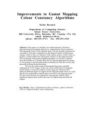
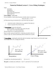
28 1. INTRODUCTIONFigure 1.15Illustration of how bias arises in using maximumlikelihood to determine the varianceof a Gaussian. The green curve showsthe true Gaussian distribution from whichdata is generated, and the three red curvesshow the Gaussian distributions obtainedby fitting to three data sets, each consistingof two data points shown in blue, usingthe maximum likelihood results (1.55)and (1.56). Averaged across the three datasets, the mean is correct, but the varianceis systematically under-estimated becauseit is measured relative to the sample meanand not relative to the true mean.(a)(b)(c)In Section 10.1.3, we shall see how this result arises automatically when we adopt aBayesian approach.Note that the bias of the maximum likelihood solution becomes less significantas the number N of data points increases, and in the limit N →∞the maximumlikelihood solution for the variance equals the true variance of the distribution thatgenerated the data. In practice, for anything other than small N, this bias will notprove to be a serious problem. However, throughout this book we shall be interestedin more complex models with many parameters, for which the bias problems associatedwith maximum likelihood will be much more severe. In fact, as we shall see,the issue of bias in maximum likelihood lies at the root of the over-fitting problemthat we encountered earlier in the context of polynomial curve fitting.Section 1.11.2.5 Curve fitting re-visitedWe have seen how the problem of polynomial curve fitting can be expressed interms of error minimization. Here we return to the curve fitting example and view itfrom a probabilistic perspective, thereby gaining some insights into error functionsand regularization, as well as taking us towards a full Bayesian treatment.The goal in the curve fitting problem is to be able to make predictions for thetarget variable t given some new value of the input variable x on the basis of a set oftraining data comprising N input values x =(x 1 ,...,x N ) T and their correspondingtarget values t =(t 1 ,...,t N ) T . We can express our uncertainty over the value ofthe target variable using a probability distribution. For this purpose, we shall assumethat, given the value of x, the corresponding value of t has a Gaussian distributionwith a mean equal to the value y(x, w) of the polynomial curve given by (1.1). Thuswe havep(t|x, w,β)=N ( t|y(x, w),β −1) (1.60)where, for consistency with the notation in later chapters, we have defined a precisionparameter β corresponding to the inverse variance of the distribution. This isillustrated schematically in Figure 1.16.
1.2. Probability Theory 29Figure 1.16 Schematic illustration of a Gaussianconditional distribution for t given x given by(1.60), in which the mean is given by the polynomialfunction y(x, w), and the precision is givenby the parameter β, which is related to the varianceby β −1 = σ 2 .ty(x 0 , w)p(t|x 0 , w,β)y(x, w)2σx 0xWe now use the training data {x, t} to determine the values of the unknownparameters w and β by maximum likelihood. If the data are assumed to be drawnindependently from the distribution (1.60), then the likelihood function is given byp(t|x, w,β)=N∏N ( t n |y(x n , w),β −1) . (1.61)n=1As we did in the case of the simple Gaussian distribution earlier, it is convenient tomaximize the logarithm of the likelihood function. Substituting for the form of theGaussian distribution, given by (1.46), we obtain the log likelihood function in theformln p(t|x, w,β)=− β N∑{y(x n , w) − t n } 2 + N 22 ln β − N ln(2π). (1.62)2n=1Consider first the determination of the maximum likelihood solution for the polynomialcoefficients, which will be denoted by w ML . These are determined by maximizing(1.62) with respect to w. For this purpose, we can omit the last two termson the right-hand side of (1.62) because they do not depend on w. Also, we notethat scaling the log likelihood by a positive constant coefficient does not alter thelocation of the maximum with respect to w, and so we can replace the coefficientβ/2 with 1/2. Finally, instead of maximizing the log likelihood, we can equivalentlyminimize the negative log likelihood. We therefore see that maximizing likelihood isequivalent, so far as determining w is concerned, to minimizing the sum-of-squareserror function defined by (1.2). Thus the sum-of-squares error function has arisen asa consequence of maximizing likelihood under the assumption of a Gaussian noisedistribution.We can also use maximum likelihood to determine the precision parameter β ofthe Gaussian conditional distribution. Maximizing (1.62) with respect to β gives1β ML= 1 NN∑{y(x n , w ML ) − t n } 2 . (1.63)n=1