Non-contact boundary layer profiler using low-coherence self ...

Exp Fluids (2007) 43:453–461DOI 10.1007/s00348-007-0320-4RESEARCH ARTICLENon-contact boundary layer profiler using low-coherenceself-referencing velocimetryAndreas Kempe Æ Stefan Schlamp Æ Thomas RösgenReceived: 18 September 2006 / Revised: 26 April 2007 / Accepted: 30 April 2007 / Published online: 21 June 2007Ó Springer-Verlag 2007Abstract A spatially self-referencing velocimetry systembased on low-coherence interferometry has been developed.The measurement technique is contactless and relieson the interference between back-reflected light from anarbitrary reference surface and seeding particles in theflow. The measurement location and the flow velocity aremeasured relative to the reference surface’s location andvelocity, respectively. Scanning of the measurement locationalong the beam direction does not require mechanicalmovement of the sensor head. The reference surface (whichcan move or vibrate relative to the sensor head) can beeither an external object or the surface of a body overwhich measurements are to be performed. The absolutespatial accuracy and the spatial resolution only depend onthe coherence length of the light source (tens of microns fora superluminescent diode). The prototype is an all-fiberassembly. An optical fiber of arbitrary length connects theself-contained optical and electronics setup to the sensorhead. Proof-of-principle measurements in water (Taylor–Couette flow) and in air (Blasius boundary layer) arereported in this paper.1 IntroductionVelocimetry techniques for boundary layer measurementsface two challenges: spatial resolution and non-intrusiveness.In most technical applications, the thickness of theA. Kempe S. Schlamp T. Rösgen (&)Institute of Fluid Dynamics, ETH Zurich,8092 Zurich, Switzerlande-mail: roesgen@ifd.mavt.ethz.chboundary layers is on the order of 1 mm such that submillimeterresolution is required for meaningful measurements.The requirements are even higher when the viscoussub-layer and the log-layer have to be resolved (Schlichtingand Gersten 2000).Traditionally, hot-wire anemometry (constant temperatureanemometry, CTA, or constant current anemometry)has been the method of choice for such measurements (e.g.,Häggmark et al. 2000; Ligrani and Bradshaw 1987; Wolffet al. 2000). The typical diameter of the wire is on theorder of micrometers. They are typically 1–2 mm long, butthe spatial resolution in the wall-parallel direction is notcritical. Because the measurement location is identical tothe probe location, the probe has to be moved to obtain thevelocity profile across the boundary layer. This makes thetechnique problematic for measurements over moving objects.But even over stationary surfaces, the thermal conductivityof the wall leads to systematic errors in themeasured velocity (Durst and Zanoun 2002; Durst et al.2001).Recently, micro-PIV has been applied to high-resolutionboundary layer measurements. PIV either requires opticalaccess from at least two directions (one for the illuminatinglaser sheet, the second for the camera) or a depth resolvingfocusing optic as in microscopy (Lin and Perlin 1998;Meinhart et al. 2000). Depending on the geometry and theobject’s movement, this might not be feasible. Laser-Doppler velocimetry (LDV) lacks the required spatialresolution, which is determined by the diameter of theintersecting laser beams and the crossing angle. LDVmeasures the velocity component perpendicular to the longaxis of the intersection ellipsoid. This means that the spatialresolution is poorest in the direction where it is mostcritical. With a novel technique using a tilted fringe system,the LDV intersection volume can also be resolved in123

454 Exp Fluids (2007) 43:453–461the order of microns (Büttner and Czarske 2001, 2003).Distributed laser Doppler velocimetry (DLDV; Gusmeroliand Martinelli 1991), a reference beam LDV using lowcoherencelight, defines the measurement location as thefocal region. The low-coherence interferometry then allowsfurther resolution within the focal region. In this respect,the technique shares many aspects with optical coherencetomography (OCT; Tomlins and Wank 2005). DLDV canbe seen as a technique similar to the approach described inthis paper.In a PIV image, the flow is visible together with theobject such that it is possible to deduce the measurementlocation (relative to the surface) from the data withoutindependent knowledge of the object’s trajectory. Nevertheless,as mentioned, the PIV installation itself might bevery challenging. CTA, LDV and DLDV on the other handhave all in common, that they are not self-referencing. Atany instance, the relative location of the object to themeasurement volume has to be known. If the motion isirregular or if the shape of the object changes over time,this might pose a problem.The new technique is self-referencing with respect to itsvertical measurement location to an arbitrary surface andhas a spatial resolution only depending on the coherencelength of the light source (e.g., see interferogram Fig. 1). Itmeasures the in-plane and out-of-plane components of thevelocity vector. The sensitivity to out-of-plane velocities(which are normally much lower) is tenfold (value can beadjusted) higher than for in-plane velocities. As for LDVand PIV, particle seeding is required. Conceptually, planarmeasurements (cf. PIV) are also possible with self-referencingcapabilities.The working principle of this new technique is explainedusing the example of a two-component boundarylayer profiler based on the Doppler effect. The systems isspatially self-referenced relative to a surface, but applicationswhere the sensor head is the reference follow thesame principle. We want to introduce a notation for thenew approach with ‘‘SR’’ standing for self-referencing, i.e.,SR-LDV.2 Measurement principleThe system consists of two main parts: the interferometerunit and the sensor head. Figure 2 shows the schematicsetup of the optical components in the interferometer unitof the system. A superluminescent diode (SLD; SuperlumDiodes Model SLD56-HP2, 1310 nm, 10 mW) emits lowcoherencelight into a single-mode fiber. The dotted line inFig. 1 is the autocorrelation function of the SLD. Thecoherence length is represented as the FMHW of the peak(~35 lm). A fiber-optical isolator protects the sensitivelight source from back-reflections and guides the light to apolarization insensitive optical circulator. The circulator isused to transfer the light through a single-mode opticalfiber to the sensor head, where a lens couples the light outof the fiber and onto the object surface.A fraction of the incident light is reflected back from thesurface of the test object onto the lens and back into thefiber towards the circulator, where it is deflected into theinterferometer. A small fraction of the light is also reflectedoff the particles passing the laser beam. Figure 3 introducesthe nomenclature used subsequently. Note that the twoincident beams are not used simultaneously (this wouldrequire a separate interferometer unit for each beam).SLDisolatorcirculatorfrom / to10.90.80.7variabledelaylinebeamsplittersensor headintensity [ ]0.60.50.4acustoopticmodulator0.30.2beamcombiner0.10−200 −150 −100 −50 0 50 100 150 200optical delay [microns]photodiodeFig. 1 Autocorrelation function of Superlum SLD-HP-56-HP: boldline simulated data based on spectrum, dotted line measurement witha freespace Michelson interferometer, dashed line measurement withthe all fiber assemblydata processing with DSO and PCFig. 2 Schematic setup of optical components in the interferometerunit, which also includes the light source123

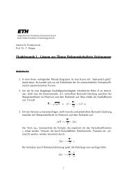
456 Exp Fluids (2007) 43:453–4613 Data analysisConsider the velocity vector u = (u,v), where u is the wallparallelvelocity and v is the wall-normal component.Assume (without loss of generality) that the bisector of thelaser beams from measurements a and b is perpendicular tothe wall (as shown in Fig. 3). Interference between rays 1aand 2a produces a peak in the power spectrum atf a ¼ 2 k ðv cos a þ u sin aÞþf AOMð1Þ(k is the wavelength of the laser beams). The Doppler shiftbetween rays 1b and 2b (from a second measurement) hasthe same magnitude, but opposite sign. The peak is thus atf b ¼ 2 k ðv cos a u sin aÞþf AOM: ð2ÞDenote the spacing of the two peaks as DF = |f a –f b | and theaverage Doppler shift as P F ¼ 1 2 ðf a þ f b Þ f AOM : Thevelocity vector is then obtained fromu ¼ kDF4sin aandv ¼ kRF2cos a :ð3ÞSince a is small, the sensitivity to wall-normal velocities(R F/v) is much larger than to in-plane velocities (DF/u). The ratio of the sensitivities is 1/tan a. This is desirable,because the wall-normal velocities are much smallerthan the wall-parallel velocities in boundary layer typeflows.4 Results4.1 Signal processingThe analog signals from the photoreceiver are first filteredby a bandpass filter (Mini Circuits BBP-60) and thenamplified by 36 dB with a high speed amplifier (HamamatsuC5594-12). The preconditioned signals are then digitizedwith 8 bit precision by a digital storage oscilloscope (DSO;LeCroy LT347L). Data is finally transferred to a PC forfurther analysis and storage. The sampling rate and theacquisition window length are set through the DSO. Thedata acquisition is triggered by a particle passing the laserbeam at the correct distance from the reference surface, i.e.,when the bandpass filtered signal exceeds a threshold (seealso Fig. 4). The dips in the unfiltered signal during relevantparticle passages (indicated by arrows) are caused by apartial blockage of ray 1 by the particle. The subsequent dataanalysis was performed by a LabView program (Ver. 7.1,National Instruments). The digitized data is first bandpassfiltered signal [mV]6050403020100−10−20−30−40−500 5 10 15 20 25 30 35 40 350time [ms]Fig. 4 Particle passages: raw signal (black) and bandpass filteredsignal (gray). The arrows indicate particle passage events (Pleasenote: The raw signal is first bandpass filtered and then amplified, thusboth signal values are not directly comparable. If the raw data weredigitized and then filtered, the beat signal would be less than thedigitizing noise)filtered with a second-order Butterworth IIR filter. Themaximum of the power spectrum is extracted by an interpolatingpeak detection routine.4.2 Taylor–Couette flowThe measurements between two coaxial rotating cylinders,i.e., Taylor–Couette flow, were performed to demonstratethe self-referencing capabilities. A metal cylinder (outerdiameter 2r i = 83 mm) was placed coaxially in the centerof a Plexiglas cylinder (inner diameter 2r o = 89.3 mm,5 mm thick). The length of both cylinders is approx.30 cm. They were installed vertically. The resulting gap, ofabout 2.85 mm, was filled with olive oil and aluminumpowder (~50 lm diameter) as seeding. The inner cylindercould rotate with frequencies of up to W/(2p) = 6 revolutionsper second.The SR-LDV sensor head was located 60 mm radiallyoutside of the outer cylinder and slightly tilted against theflow direction. Due to the beam deflections at the curvedPlexiglas surface, the angle of incidence relative to theinner cylinder is not known a priori. It was later calculatedbased on the measured frequency shifts near the wall andthe known rotation rate (15°). For these flow parametersthe flow is laminar and the flow is parallel such that thewall-normal velocity component is known to be zero.Measurements with a single incidence angle are thus sufficient.A retro-reflecting foil was attached to the inner cylinder(the reference surface). The primary reason for this was toincrease the reflection level from the reference surface backinto the collimator lens. The reflections from the metalcylinder are otherwise very directional and thus largely620570510460405raw signal [mV]123

458 Exp Fluids (2007) 43:453–461Us − relative error [%]8765432100 0.2 0.4 0.6 0.8 1 1.2 1.4 1.6surement window of 25K samples. At the highest rotationalspeed only 5,000 samples have been recorded. The spectralresolution was 2 and 10 kHz, respectively.The spatially periodic structure of the retro-reflectormoving with the rotating cylinder caused a temporallyperiodic signature in the recorded signal. Because thismodulation was well outside the expected frequency rangefrom interfering beams (f AOM ± DF), it could be discriminatedfrom the useful signals. It did, however, limit thelength over which a single particle passage produces acontinuous interference signal. When measuring close tothe stationary wall, this modulation limited the duration ofthe signature of a particle passage. Consequently, theacquisition window was set approximately to this value.At higher rotational speeds the beat signal length wasshorter than the acquisition window, which means that theeffective real spectral resolution was lower than the theoreticalvalue for a given frequency and the length of theacquisition window. Hence, at the highest surface speed of1.55 m/s, a shorter acquisition window was used such thatthe beat signal lengths were again comparable to theacquisition window.4.3 Blasius boundary layermean standard deviationmax positive errormax negative errorsurface velocity [m/s]Fig. 7 SR-LDV measured Taylor–Couette flow profiles; range anduncertainty of data relative to wall speed of rotating cylinderWith a more powerful SLD (Exalos, EXS1320-1111,1320 nm, 25 mW) it was also possible to perform measurementsin air. For these feasibility tests the boundarylayer profile over a flat plate was measured. An aluminumsharp edge, approx. 70 mm wide, 30 mm long and 1 mmthick was installed horizontally inside a small wind tunnel.As seeding particles small salt crystals with a diameter ofapprox. 3 lm were used. They were generated by anultrasonic atomizer within a water–salt solution (Ruschet al. 2007) and then injected in front of the wind tunnelinlet. To avoid contamination of the laboratory with the saltparticles, the open loop wind tunnel discharged into a 5 mlong flexible pipe guiding the exhaust air to a vent.Optical access was provided through a clear adhesivetape. The tape was stretched across a port hole in the tunnelwall, measuring approx. 30 mm · 80 mm (see Fig. 8). Theoptical sensor head, a focusing lens with a diameter ofabout 5 mm, was installed above this window at a distanceof 6 cm to the aluminum plate.The focal point of the laser was set close to the surfaceof the flat plate, simply by focusing until the highest surfacereflection could be achieved. The aluminum surfacewas slightly roughened in order to obtain good reflectionsback into the collection lens even at higher incidence angles.Figure 9 shows the boundary layer profiles measured atthree different flow speeds. The plotted data represents themean value of approx. 20 particle passages for each verticalposition. The reference flow rates were measured witha conventional propeller velocimeter (Schiltknecht, modelnumber 12675). The measurement position was 6 mmdownstream of the leading edge on the upper side of theplate. The incidence angle was set to ±15° (‘‘forward’’ and° “15 backwardsetup”flow directionoptical access throughclear adhesive tape°“15 forwardsetup”Fig. 8 Optical access to the sharp edge flat plate in the wind tunnel isprovided through clear adhesive tapewall normal position [microns]200018001600140012001000800600400200u (U=1.7 m/s)10 x vu (U=2.5 m/s)10 x vu (U=3.65 m/s)10 x vBlasius theory00 0.5 1 1.5 2 2.5 3 3.5 4velocity [m/s]Fig. 9 Measured and theoretical Blasius profiles. (U = 1.7,2.5,3.65 m/s,Re x = 680,1000,1400)123

Exp Fluids (2007) 43:453–461 459‘‘backward’’ measurement setups). After measuring allthree flow rates in the forward setup, the sensor head wasrotated to the backward setup. In order to investigate thesame downstream position on the flat plate, a repositioningof the sensor head was hence necessary.It can be seen that the measured data is in very goodagreement with the Blasius theory. It has to be said that thefreestream velocity input (measured with the propellermeter) for the theoretical profile calculation was slightlychanged (maximum by ±0.1 m/s), in order to achieve thebest fit with the measured profile. Nevertheless, for thewall-parallel velocity component, only a few points show asmall deviation from the theoretical boundary layer shape(±1%). Agreement for the out-of-plane velocity (scaled upin the plot by a factor of 10) is worse, but still satisfactory.Note that the measurement uncertainty (in absolute terms)is independent of the flow velocity. This leads to largerelative errors for low flow velocities.In contrast to the measurements in liquid, no retroreflectingfoil was used to generate the reference reflection.Hence, the zero delay setting of the interferometer is equalto the zero wall normal position. As mentioned before, formeasurements very close to the surface this leads to largebeat signal due to interference of each signal with itself.Therefore, measurements within the first 150 lm above thesurface could not be obtained. Since this value only dependson the light source, but is independent of the flow,the spatial resolution in terms of wall units will depend onthe flow. For the intermediate flow speed of U = 2.5 m/s(Re x = 1000), this corresponds to y + 3.5. If desired, itwould also be possible to use a retro-reflector in gaseousflows, allowing measurements much closer to the wall.5 Measurement uncertainty considerations5.1 General measurement precisionEven though various error sources for LDV are discussed inthe literature (e.g., Durst et al. 1987, and references giventherein), the overall measurement error for a specific systemand for a specific application is not easy to estimate. Inaddition, to validate a new LDV sensor concept a simpletheoretical model might not be feasible. Alternatively, validationsare done experimentally by measuring a well-knownphenomenon and comparing the results with the theory.For this novel boundary layer profiler this was done witha number of generic flows, i.e., a Poiseuille flow, a Taylor–Couette flow and a laminar Blasius boundary layer. Theestimation of the errors in these specific experiments wasdone under the assumption of a theoretical perfect flow (noturbulence). To make the results comparable, the opticalarrangement of the sensor head was not modified (lensdiameter 5 mm, measurement distance approx. 60 mm,observation angle ±15°).In general, a simple lower limit for the frequencymeasurement accuracy can be given byDf min 1 Dt ;ð5Þwhere Dt is the length of the observed particle burst. Thiscould be improved by a factor of about 2 due to theinterpolation scheme for the peak detection in the powerspectrum. However, this value strongly depends on theexperimental setup and cannot be taken as constant. In thefollowing only two sources of error are described, whichare significant for the self-referencing setup.5.2 Aperture broadeningAs shown in Fig. 10, the angle of scattered light can varyfrom a–b to a + b depending on the aperture of the collectinglens. Since the Doppler shift of the backscattered light amongothers also depends on the observation angle, this results in abroadening of the received Doppler frequency signal. In afirst estimate (see, Saarimaa 1979, for experimental validation)the limits of this effect can be determined asDf broad ¼ 2u sin b:k ð6ÞThe mean Doppler shift for a reference beam LDV dependson the incidence angle aDf mean ¼ 2u sin a:k ð7ÞThe ratio of the broadening effect and the mean Dopplershift is then- /2surfacecollectinglensFig. 10 Aperture broadening through finite collection angle 2b andshadowing effect through partial blockage of the aperture by passingparticles123

460 Exp Fluids (2007) 43:453–461f broad ¼ sin bsin a :ð8ÞTaking the mean Doppler shift as the quantity of interestfor flow velocity measurements, this ratio can be seen asthe maximum impact factor of aperture broadening ontothe measurement value.5.3 Shadowing effectThe shadowing effect is specific to self-referencing LDV.Since the reflection from the particle and reference surfaceare in line outside of the interferometer, a particle crossingthe laser beam can partially hide the reflections of thesurface during its passage (see Fig. 4). To make a selfreferencedmeasurement, the light from the particle andfrom the surface has to interfere to generate a signal. Incase of interference, a relatively large signal from thesurface can act as an amplifier for the beat note. Therefore,one has to make sure that while a particle passes the focus,sufficient surface reflections are also visible.There are also consequences for the measured velocity.Consider a particle passing through the shaded region inFig. 10. The particle will reflect light symmetrically backonto the lens. The broadening will then be as given inEq. 6. At the same time, the particle blocks parts of the lensfor light reflected by the surface. The effective collectionangle is thus less than 2b and the mean angle is not a, buta–b/2 (neglecting that the lens is spherical and assumingthat one half of the lens is blocked completely).In case of a moving surface this leads to a shifted beatsignal and in turn to a false measurement of the velocitydifference between surface and particle. In contrast to theaperture broadening, this effect cannot be compensated byan interpolation mechanism for the frequency determination.The absolute frequency error scales with b, but therelative error scales like that for the broadening effect(Eq. 8).6 ConclusionsAn optical velocimetry technique was presented which isbased on low-coherence interferometry. The extent and theerror of the location of the measurement volume is comparableto the coherence length of the light source (tens ofmicrometers). The measurement location is set relative to areference surface (which could be the surface of a movingobject). The measurement location can be scanned along aline without mechanical movement of the sensor head. Asfor standard LDV techniques particle seeding is necessary.Multiple components of the velocity vector can be measuredusing a single interferometer and light source. Thiscan be achieved by either taking measurements subsequentlyfrom different directions or by a multi-beam setup.A multi-beam setup can take advantage of the fact that thesame light source can be used for all velocity components,but that a separate interferometer is required for eachobservation direction. This, in turn, requires a separatecollection lens for each direction and thus a separate fiber.The data rate depends on the number of particlescrossing the sample volume per unit time. It is thus proportionalto the seeding density, but also to the flowvelocity and inversely proportional to the extent of thesample volume in each direction. There hence exists atrade-off between spatial resolution and data rate. In themeasurements presented in Sec. 4, the data rate was onlyone particle passage every few seconds. Even at higherseeding densities or flow velocities, turbulent time scalescan clearly not be resolved. Yet, histograms for the velocitiycan be accumulated over time.The measurement range depends on the power of thelight source, the reflection levels of the reference surfaceand the particles (i.e., particle size), and the collectionangle of the optics (i.e., lens diameter and distance to themeasurement volume). In the first test series, a lens with adiameter of 5 mm, a measurement distance of 60 mm(collection angle of approx. 5°), aluminum powder asparticle seeding (approx. 50 lm diameter) and a 10 mWlight source were used. This allowed a measurement rangeof approx. 4 mm, without moving the sensor head.Improvements could be made using a more powerful lightsource. For measurements in liquids the measurementrange was increased by a factor of 2. Hence, the focal pointdoes not need to be exactly at the surface, which facilitatesthe handling of the sensor. With the increase in light power,measurements in air could also be demonstrated. With acollection angle of approx. 5° and small salt crystalsas seeding (1–4 lm diameter) a measurement range ofapprox. 2 mm without relocating the sensor head waspossible.Decreasing the collection angle leads to an elongatedfocal point, which in turn increases the range in which thesensor front end does not need to be moved to collectparticle reflections, as well as the absolute measurementrange in respect to the surface (i.e., the region where enoughsurface reflections are available). It also increases theaccuracy of the velocity measurement, due to longer passagetimes. On the other hand it significantly reduces thereflection level from the particles. Due to the autocorrelatorsetup of the interferometer and the large zero delay signal,measurements within the first 150 lm above the wall couldnot be performed directly, but only by using a retroreflectingfoil.Further developments will focus on the handling of thesensor. Although the sensor has self-referencing capabili-123

Exp Fluids (2007) 43:453–461 461ties, measurements are only possible when the focus is setclose to the surface, especially when using small particlesas in air flows. To overcome this limitation an autofocusingoptic will be implemented. Furthermore, with theactual SR-LDV single beam setup the incidence angle tothe surface must be known, which is a direct source ofuncertainty. With a SR-LDV dual-beam configuration theangle of incidence would be inherently known. This setupalso adds a general interferometer offset, which makes theretro-reflector obsolete and which directly allows for 1-dimensional, 2-component measurements (without rotatingthe sensor head as in single beam SR-LDV). Additionalprovisions can be made to adapt the system to 2-dimensional,2-component measurements by the use of a planarsurface scanning technique.ReferencesBüttner L, Czarske J (2001) A multimode-fiber laser-Doppleranemometer for highly spatially resolved velocity measurementsusing low-coherence light. Measurements Science and Technology12:1891–1903Büttner L, Czarske L (2003) Spatial resolving laser Doppler velocityprofile sensor using slightly tilted fringe systems and phaseevaluation. Measurement Science and Technology 14:2111–2120Durst F, Zanoun ES (2002) Experimental investigation of near-walleffects on hot-wire measurements. Experiments in Fluids33(1):210–218Durst F, Melling A, Whitelaw JH (1987) Theorie und Praxis derLaser-Doppler-Anemometrie. Braun, KarlsruheDurst F, Zanoun ES, Pashtrapanska M (2001) In situ calibration of hotwires close to highly heat-conducting walls. Experiments inFluids 31(1):103–110Gusmeroli V, Martinelli M (1991) Distributed laser Dopplervelocimeter. Optics Letters 16(17):1358–1360Häggmark CP, Bakchinov AA, Alfredsson PH (2000) Measurementswith a flow direction boundary-layer probe in a two-dimensionallaminar separation bubble. Exp Fluids 28:236–242Ligrani PM, Bradshaw PH (1987) Spatial resolution and measurementof turbulence in the viscous sublayer using subminiature hotwireprobes. Exp Fluids 5:407–417Lin HJ, Perlin M (1998) Improved methods for thin, surface boundarylayer investigations. Exp Fluids 25:431–444Meinhart CD, Wereley ST, Gray MHB (2000) Volume illuminationfor two-dimensional particle image velocimetry. MeasurementsScience and Technology 11:809–814Rusch D, Kempe A, Rösgen T (2007) Seeding of high temperature airflow. Exp Fluids 42:761–765Saarimaa R (1979) A laser Doppler velocimeter for surface velocitymeasurement. Journal of Physics E 12:600–603Schlichting H, Gersten K (2000) Boundary-Layer Theory. SpringerVerlag, BerlinTomlins PH, Wank RK (2005) Theory, developments and applicationsof optical coherence tomography. Journal of Physics D38(15):2519–2535Wolff S, Brunner S, Fottner L (2000) The use of hot-wireanemometry to investigate unsteady wake-induced boundarylayerdevelopment on a high-lift lp turbine cascade. Journal ofTurbomachinary 122:644–650123