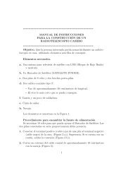
where the 0 z i # (m) terms are the phase averages from the triply extended subsequence, and the prefix 0 denotes that thelinear trend has been removed. At the largest possible averaging factor, m = N/3, the outer summation consists <strong>of</strong>only one term, but the inner summation has 6m terms, thus providing a sizable number <strong>of</strong> estimates for the variance.Reference for Modified Total VarianceD.A. Howe and F. Vernotte, “Generalization <strong>of</strong> the Total Variance Approach to the Modified Allan Variance,” Proc.31 st PTTI Meeting, pp. 267-276, Dec. 1999.5.2.13. Time Total VarianceThe time total variance, TTOT, is a similar measure <strong>of</strong> time stability, based on themodified total variance. It is defined as32 τ2σx( τ) = ⋅ Modσtotal( τ )(28)3The time total variance is ameasure <strong>of</strong> time stabilitybased on the modified totalvariance.5.2.14. Hadamard Total VarianceThe Hadamard total variance, HTOT, is a total version <strong>of</strong> the Hadamard variance.As such, it rejects linear frequency drift while <strong>of</strong>fering improved confidence at largeaveraging factors.An HTOT calculation begins with an array <strong>of</strong> N fractional frequency data points, y iwith sampling period τ 0 that are to be analyzed at averaging time τ =m τ 0. HTOT iscomputed from a set <strong>of</strong> N − 3m + 1 subsequences <strong>of</strong> 3m points. First, a linear trend(frequency drift) is removed from the subsequence by averaging the first and lasthalves <strong>of</strong> the subsequence and dividing by half the interval. Then the drift-removedThe Hadamard total variancecombines the features <strong>of</strong> theHadamard and total variancesby rejecting linear frequencydrift, handling more divergentnoise types, and providingbetter confidence at largeaveraging factors.subsequence is extended at both ends by uninverted, even reflection. Next the Hadamard variance is computed forthese 9m points. Finally, these steps are repeated for each <strong>of</strong> the N − 3m + 1 subsequences, calculating HTOT as theiroverall average. These steps are shown in Figure11.26
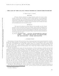
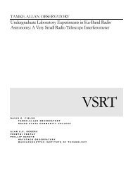
Fractional <strong>Frequency</strong> Data y i, i = 1 to NN-3m+1 Subsequences:3my ii=n to n+3m-1Linear Freq Drift Removed:0 y i y i= y i- c i ⋅ i, c i= freq drift9mExtended Subsequence: 0 y # n-l= 0 y n+l-1 0 y # i 0 y # n+3m+l-1=Uninverted, Even Reflection:0 y n+3m-l1 ≤ l ≤ 3m9 m-Point Averages:6m 2nd Differences:Had σ 2Calculate Had σ 2 y (τ) = 1/6 ⋅ 〈 z 2 n(m) 〉, wherey (τ) for Subsequence: _ _ _z n(m) = y n(m) - 2y n+m(m) + y n+2m(m)Then Find HTOT as Average <strong>of</strong> SubestimatesFigure 11. Steps to calculate Hadamard Total Variance.Computationally, the HTOT process requires three nested loops:• An outer summation over the N − 3m + 1 subsequences. The 3m-point subsequence is formed, its linear trend isremoved, and it is extended at both ends by uninverted, even reflection to 9m points.• An inner summation over the 6m unique groups <strong>of</strong> m-point averages from which all possible fully overlappingsecond differences are used to calculate HVAR.• A loop within the inner summation to sum the frequency averages for three sets <strong>of</strong> m points.The final step is to scale the result according to the sampling period, τ 0 , averaging factor, m, and number <strong>of</strong> points, N.Overall, this can be expressed as:N− 3m+ 1 n+ 3m−12 1 ⎛ 12 ⎞TotalHσy ( m, τ0, N ) = ( Hi( m))6( N − 3m+ 1)⎜n= 1 6m⎟⎝ i= n−3m⎠∑ ∑ , (29)where the H i (m) terms are the z n (m) Hadamard second differences from the triply extended, drift-removedsubsequences. At the largest possible averaging factor, m = N/3, the outer summation consists <strong>of</strong> only one term, butthe inner summation has 6m terms, thus providing a sizable number <strong>of</strong> estimates for the variance. The Hadamardtotal variance is a biased estimator <strong>of</strong> the Hadamard variance, so a bias correction is required that is dependent on thepower law noise type and number <strong>of</strong> samples.The following plots shown the improvement in the consistency <strong>of</strong> the overlapping Hadamard deviation resultscompared with the normal Hadamard deviation, and the extended averaging factor range provided by the Hadamardtotal deviation [10].27
- Page 1 and 2: NIST Special Publication 1065Handbo
- Page 3 and 4: NIST Special Publication 1065Handbo
- Page 6 and 7: PrefaceI have had the great privile
- Page 8 and 9: 5.12. MTOT BIAS FUNCTION ..........
- Page 11 and 12: 1 IntroductionThis handbook describ
- Page 13 and 14: Original Allan (a)Overlapping Allan
- Page 15 and 16: 3 Definitions and TerminologyThe fi
- Page 17 and 18: 15000Random Run Noise50Random Walk
- Page 19 and 20: 5 Time Domain StabilityThe stabilit
- Page 21 and 22: step) are the sample period τ 0 an
- Page 23 and 24: (a)(c)(b)Figure 5. (a) Simulated fr
- Page 25 and 26: In terms of phase data, the Allan v
- Page 27 and 28: 22 df ⋅ sχ = , (12)2σwhere χ²
- Page 29 and 30: References for Time Variance1. D.W.
- Page 31 and 32: M− 3m+1 j+ m−121⎧⎫Hσy( τ)
- Page 33 and 34: References for Hadamard Variance1.
- Page 35: 5.2.12. Modified Total VarianceThe
- Page 39 and 40: It is necessary to identify the dom
- Page 41 and 42: NoiseRW FMTable 3. Thêo1 EDF Formu
- Page 43 and 44: References for Thêo1, NewThêo1, T
- Page 45 and 46: where S φ is the spectral density
- Page 47 and 48: References for Dynamic Stability1.
- Page 49 and 50: 1000100N=500250100Full EDF Algorith
- Page 51 and 52: The edf for the modified Allan vari
- Page 53 and 54: References for Confidence Intervals
- Page 55 and 56: 5.5.4. The Lag 1 AutocorrelationThe
- Page 57 and 58: The input data should be for the pa
- Page 59 and 60: 5.9. B 3 Bias FunctionThe B 3 bias
- Page 61 and 62: References for Bias Functions1. “
- Page 63 and 64: Figure 24. Frequency stability plot
- Page 65 and 66: include points at all possible tau
- Page 67 and 68: x(t) = a + bt, where slope = y(t) =
- Page 69 and 70: Linear frequency drift can be estim
- Page 71 and 72: References for Environmental Sensit
- Page 73 and 74: AllandeviationHadamarddeviationTota
- Page 75 and 76: For πτf
- Page 78 and 79: S(f)yS(f)=x, (59)(2π f)2where S x
- Page 80 and 81: preferred, either because of measur
- Page 82 and 83: References for Spectral Analysis1.
- Page 84 and 85: where the h α terms define the lev
- Page 86 and 87:
The expected PSD values that corres
- Page 88 and 89:
8.1. White Noise GenerationWhite no
- Page 90 and 91:
9 Measuring SystemsFrequency measur
- Page 92 and 93:
factor. For example, if two 5 MHz s
- Page 94 and 95:
Figure 37. Random telegraph signal
- Page 96 and 97:
10 Analysis ProcedureA frequency st
- Page 98 and 99:
5 Remove the frequencydrift, leavin
- Page 100 and 101:
10.4. Gap HandlingGaps should be in
- Page 102 and 103:
References for Gaps, Jumps, and Out
- Page 104 and 105:
Table 23. Stability data for unit u
- Page 106 and 107:
B1 ⎡ ⎤∑∑− , (72)⎣ ⎦M
- Page 108 and 109:
The total deviation canprovide bett
- Page 110 and 111:
The Hadamard variance isinsensitive
- Page 112 and 113:
Table 28. Detection of periodic com
- Page 114 and 115:
11.6. White FM Noise of a Frequency
- Page 116 and 117:
12 SoftwareSoftware is necessary to
- Page 118 and 119:
This expression produces a series o
- Page 120 and 121:
13 GlossaryThe following terms are
- Page 122 and 123:
14 Bibliography• NotesA. These re
- Page 124 and 125:
44. P. Lesage and T. Ayi, “Charac
- Page 126 and 127:
81. J. McGee and D.A. Howe, “Thê
- Page 128 and 129:
• Noise Identification122. J.A. B
- Page 130 and 131:
162. W.J. Riley, “Addendum to a T
- Page 132 and 133:
OOutlier . 41, 75, 106, 108, 109, 1
- Page 135 and 136:
NIST Technical PublicationsPeriodic