Handbook of Frequency Stability Analysis

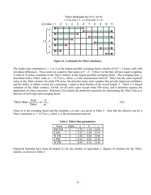
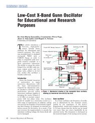
x[ ] index =01Theo1 Schematic for n=11, m=10i =1 to n-m = 1 , δ = 0 to m/2 -1 = 41 2 3 4 5 6 7 8 9 10 11δ234Figure 14. A schematic for Thêo1 calculation.The single outer summation (i = 1 to 1) at the largest possible averaging factor consists of m/2 = 5 terms, each withtwo phase differences. These terms are scaled by their spans m/2 − δ = 5 thru 1 so that they all have equal weighting.A total of 10 terms contribute to the Theo1 statistic at this largest-possible averaging factor. The averaging time, τ,associated with a Thêo1 value is τ = 0.75·m·τ 0 , where τ 0 is the measurement interval. Thêo1 has the same expectedvalue as the Allan variance for white FM noise, but provides many more samples that provide improved confidenceand the ability to obtain a result for a maximum τ equal to three-fourths of the record length, T. Thêo1 is a biasedestimator of the Allan variance, AVAR, for all noise types except white FM noise, and it therefore requires theapplication of a bias correction. Reference [2] contains the preferred expression for determining the Thêo1 bias as afunction of noise type and averaging factor:Avar bThêo1 Bias= = a+ , (31)cThêo1 mwhere m is the averaging factor and the constants a, b and c are given in Table 2. Note that the effective tau for aThêo1 estimation is τ = 0.75·m·τ 0 , where τ 0 is the measurement interval.Table 2. Thêo1 bias parameters.Noise Alpha a b cRW FM −2 2.70 −1.53 0.85F FM −1 1.87 −1.05 0.79W FM 0 1.00 0.00 0.00F PM 1 0.14 0.82 0.30W PM 2 0.09 0.74 0.40Empirical formulae have been developed [1] for the number of equivalent χ 2 degrees of freedom for the Thêo1statistic, as shown in Table 3:30