Handbook of Frequency Stability Analysis

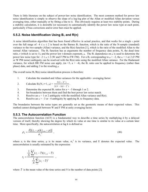
There is little literature on the subject of power-law noise identification. The most common method for power lawnoise identification is simply to observe the slope of a log-log plot of the Allan or modified Allan deviation versusaveraging time, either manually or by fitting a line to it. This obviously requires at least two stability points. Duringa stability calculation, it is desirable (or necessary) to automatically identify the power law noise type at each point,particularly if bias corrections and/or error bars must be applied.5.5.2. Noise Identification Using B 1 and R(n)A noise identification algorithm that has been found effective in actual practice, and that works for a single τ pointover the full range of –4 ≤ α ≤ 2 is based on the Barnes B 1 function, which is the ratio of the N-sample (standard)variance to the two-sample (Allan) variance, and the R(n) function [1], which is the ratio of the modified Allan to thenormal Allan variances. The B 1 function has as arguments the number of frequency data points, N, the dead timeratio, r (which is set to 1), and the power law t-domain exponent, μ. The B 1 dependence on μ is used to determine thepower law noise type for –2 ≤ μ ≤ 2 (W and F PM to FW FM). For a B 1 corresponding to μ = –2, the α = 1 or 2 (F PMor W PM noise) ambiguity can be resolved with the R(n) ratio using the modified Allan variance. For the Hadamardvariance, for which RR FM noise can apply, (m =3, a = –4), the B 1 ratio can be applied to frequency (rather thanphase) data, and adding 2 to the resulting μ.The overall noise B 1 /R(n) noise identification process is therefore:1. Calculate the standard and Allan variances for the applicable τ averaging factor.2. Calculate B 1 (N, r=1, μ) =μN( 1 − N ).μ2( N −1)( 1−2 )3. Determine the expected B 1 ratios for a = –3 through 1 or 2.4. Set boundaries between them and find the best power law noise match.5. Resolve an α = 1 or 2 ambiguity with the modified Allan variance and R(n).6. Resolve an α = –3 or –4 ambiguity by applying B 1 to frequency data.The boundaries between the noise types are generally set as the geometric means of their expected values. Thismethod cannot distinguish between W and F PM at unity averaging factor.5.5.3. The Autocorrelation FunctionThe autocorrelation function (ACF) is a fundamental way to describe a time series by multiplying it by a delayedversion of itself, thereby showing the degree by which its value at one time is similar to its value at a certain latertime. More specifically, the autocorrelation at lag k is defined asρ =kE[( zt−μ)( zt+k−μ)]2, (46)σzwhere z t is the time series, μ is its mean value, σ 2zautocorrelation is usually estimated by the expressionis its variance, and E denotes the expected value. Therk=1NN−k∑t=11N( z −z)( z −z)tN∑t=1t+k( z − z)t2, (47)where z is the mean value of the time series and N is the number of data points [2].44