A General Approach to Real Option Valuation with ... - ICMA Centre

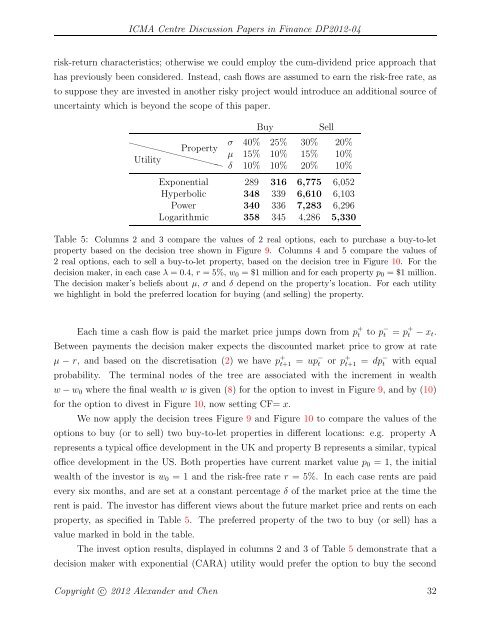
ICMA Centre Discussion Papers in Finance DP2012-04risk-return characteristics; otherwise we could employ the cum-dividend price approach thathas previously been considered. Instead, cash flows are assumed to earn the risk-free rate, asto suppose they are invested in another risky project would introduce an additional source ofuncertainty which is beyond the scope of this paper.❳ ❳❳❳ ❳❳❳ PropertyUtility ❳ ❳❳❳❳BuySellσ 40% 25% 30% 20%μ 15% 10% 15% 10%δ 10% 10% 20% 10%Exponential 289 316 6,775 6,052Hyperbolic 348 339 6,610 6,103Power 340 336 7,283 6,296Logarithmic 358 345 4,286 5,330Table 5: Columns 2 and 3 compare the values of 2 real options, each to purchase a buy-to-letproperty based on the decision tree shown in Figure 9. Columns 4 and 5 compare the values of2 real options, each to sell a buy-to-let property, based on the decision tree in Figure 10. For thedecision maker, in each case λ =0.4, r =5%,w 0 = $1 million and for each property p 0 = $1 million.The decision maker’s beliefs about μ, σ and δ depend on the property’s location. For each utilitywe highlight in bold the preferred location for buying (and selling) the property.Each time a cash flow is paid the market price jumps down from p + t to p − t = p + t − x t .Between payments the decision maker expects the discounted market price to grow at rateμ − r, and based on the discretisation (2) wehavep + t+1 = up− t or p + t+1 = dp− t with equalprobability. The terminal nodes of the tree are associated with the increment in wealthw − w 0 where the final wealth w is given (8) for the option to invest in Figure 9, andby(10)for the option to divest in Figure 10, now setting CF= x.We now apply the decision trees Figure 9 and Figure 10 to compare the values of theoptions to buy (or to sell) two buy-to-let properties in different locations: e.g. property Arepresents a typical office development in the UK and property B represents a similar, typicaloffice development in the US. Both properties have current market value p 0 = 1, the initialwealth of the investor is w 0 = 1 and the risk-free rate r = 5%. In each case rents are paidevery six months, and are set at a constant percentage δ of the market price at the time therent is paid. The investor has different views about the future market price and rents on eachproperty, as specified in Table 5. The preferred property of the two to buy (or sell) has avalue marked in bold in the table.The invest option results, displayed in columns 2 and 3 of Table 5 demonstrate that adecision maker with exponential (CARA) utility would prefer the option to buy the secondCopyright c○ 2012 Alexander and Chen 32