JLAB-TN-03-003 (2003) - JLab Tech Notes Home Page - Jefferson ...

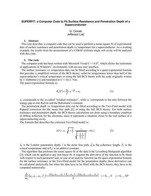
SUPERFIT: a Computer Code to Fit Surface Resistance and Penetration Depth of aSuperconductorG. CiovatiJefferson Lab1. AbstractThis note describes a computer code that can be used to perform a mean-square fit of experimentaldata of surface resistance and penetration depth vs. temperature for a superconductor. As a workingexample, the results from the measurement of a CEBAF niobium single cell cavity will be analysedwith this code.2. The codeThe computer code has been written with Microsoft Visual C++ 6.0 © , which allows the realizationof applications in Windows © environment, with an easy user interface.The surface resistance vs. temperature data can be fitted according to a quasi-exponential formulathat provides a simplified version of the BCS theory, valid for temperatures lower than half of thesuperconductor’s critical temperature or using the full BCS theory with the code originally writtenby J. Halbritter [1] and translated in C++ by J. Yan.The quasi-exponential formula is:RaT0 −a1 T( T ) = ⋅ea2S+(1)a 2 corresponds to the so-called “residual resistance”, while a 1 corresponds to the ratio between theenergy gap at zero Kelvin and the Boltzmann’s constant.The penetration depth vs. temperature data can be fitted according to the Two-Fluid model withPippard correction for the mean free path [2] or using the full BCS theory. For both surfaceresistance and penetration depth, the BCS theory calculations are done using a boundary conditionof diffuse reflection for the electrons, since it represents a situation closer to the real surface of asuperconducting cavity.The formula that describes the corrected Two-Fluid model is:λ1( T ) = λ ⋅ 1 + ⋅− λ( T )(2)Lξl⎛ T ⎞1 − ⎜ ⎟T⎝ C ⎠λ L is the London penetration depth, l is the mean free path, ξ is the coherence length, T C is thecritical temperature and λ(T 0 ) is an additive constant.The algorithm that performs the mean square fit of the data is the Levenberg-Malquardt algorithm[3], which can be applied to any non-linear fit. It requires the derivative of the function to be fittedwith respect to each parameter and, in case of an analytic function (as the quasi-exponential formulafor the surface resistance or the Two-Fluid model for the penetration depth), these derivatives canbe calculated analytically but when the data have to be fitted with the BCS theory, they have to becomputed numerically:dydaiy(a0,a1,...,ai+ hi,... aN) − y(a0,a1,...,ai,... aN)( a , a ,... a , T ) =i = 0,..., N j 0,..., NP0 1 N j=hi40

for each parameter a i and temperature value T j . The increment h has been chosen to be 5% of theparameter’s value.As for any non-linear fit, the initial guess value for the parameters is very important to improvethe goodness of fit, since initial values too far from the solution may result in an higher chi-squaredor a non-convergent calculation. In general, it’s a good idea to run the program with initial valuesequal to the ones resulted from a first fit of the same data.There exists a version of the code that runs on a DOS shell and, if compiled with a Linux C++compiler, can run on a Linux machine as well. The Windows © version has been called WinSuperfit.3. Superfit manual and exampleThis section describes the feature of the Windows version of the program.When the program is launched, two warning messages appear, regarding a library that has beenused in the program and is not registered. Just click the “OK” button after few seconds.Figure 1: Main program windowThe main window shows the four choices to fit surface resistance or penetration depth vs.temperature data. Just click the option you would like to run. Depending on the selected option, anew window appears. On the left there are all the required parameters and a box to be checked if theparameter can be changed during the fit. The default parameters values correspond to niobium.

Figure 2: Window for fitting penetration deoth vs. temperature data with BCS theory.The input data are loaded by pressing the “Open File” button and selecting the filename. It has tobe an ASCII file (for example a text file) that begins with the number of data points followed bytwo or three columns of data, the first one being the temperature values in Kelvin, the second onebeing the surface resistance (in ohm) or penetration depth (in Angstrom) data. The third column isfacultative and contains the experimental error for each data point. The input file can be easilycreated with Excel. The maximum number of data points is 500.Temperature values17Number of points3.047 1.71053E-072.976 1.65756E-072.9 1.44139E-072.853 1.36024E-072.804 1.25981E-072.705 1.03136E-072.651 1.00073E-072.497 7.90617E-082.425 7.49382E-08 Surface resistance values2.302 5.4242E-082.204 5.04435E-082.087 3.85375E-082.046 3.5888E-081.987 3.26048E-081.938 2.91698E-081.884 2.80778E-081.843 2.66602E-08Figure 3: Example of input file

The program then asks if the measurement errors (third column) is included or not in the input file.In case it is, the “Measurement error” field is disabled; otherwise one can set a percentage value forit. The “Calculation accuracy” field refers to the accuracy with which the BCS theory calculationsneed to be done.Once the data are loaded, a “guess” value for the parameters has been assigned and it has beendecided which parameters to fit for, the “Fit” button becomes enabled. By pressing it the meansquarefit algorithm starts. The results are shown on the right side of the window.Fitting data using the BCS theory takes a lot of time and CPU capability, and the results from eachiteration step are shown at the bottom of the window. These include the iteration number, the chisquare,the parameter “alamda”, which is an indication of the variation applied to the fittingparameters, and finally the fitting parameters a i (i = 0,1...5) corresponding to the input parameterslisted from top to bottom. The calculations can be stopped at any time by pressing the “Exit” buttonand then the “Quit” button in the main window.Figure 4: Window look after fitting penetration depth vs. temperature data with Two-Fluid modelOnce the fitting process is completed, the “Plot” button is enabled and allows creating a plot ofthe input data along with a curve describing the fitted function. The plot function has been doneusing a graphic library included in the book in ref. [4].

Figure 5: Window that shows input data and fitted functionPressing the “Save File” button, it is possible to save the initial parameters values, the values afterthe fit with the chi-square, the input data along with the data obtained from the fitted function andfinally the experimental errors.For example, in figure 6 are shown the results from a fit of the variation of penetration depth withtemperature on a CEBAF niobium single cell cavity using the Two-Fluid model. The parametersthat could be adjusted during the fit had been chosen to be the critical temperature, the mean freepath, the London penetration depth and the additive constant.Result from fitting Penetration Depth vs. T with two-fluid modelInitial parameters:Critical temperature (a1) [K] = 9.442London penetration depth (a2) [A] = 387Coherence length (a3) [A] = 620Mean free path (a4) [A] = 493Penetration depth at 0 K (a5) [A] = 610chi-squared = 89.9298a1 = 9.44219 +/- 0.00553882a2 = 386.993 +/- 400186a4 = 493.032 +/- 1.83054e+006a5 = 609.997 +/- 6.25004T [K] Lambda [A] Lambda fit [A] stdev [A]5.205 0.321 0.323 0.0165.510 11.543 8.423 0.577

T [K] Lambda [A] Lambda fit [A] stdev [A]5.830 24.048 18.962 1.2026.120 33.988 30.747 1.6996.375 41.683 43.284 2.0846.605 48.096 56.738 2.4056.850 67.013 73.834 3.3516.900 72.785 77.733 3.6396.950 77.274 81.789 3.8647.000 83.686 86.007 4.1847.050 88.496 90.398 4.4257.105 92.023 95.438 4.6017.160 96.512 100.710 4.8267.210 103.245 105.718 5.1627.265 108.055 111.476 5.4037.310 111.582 116.393 5.5797.370 116.392 123.257 5.8207.420 121.522 129.263 6.0767.475 130.820 136.190 6.5417.525 140.760 142.799 7.0387.580 150.700 150.437 7.5357.640 158.395 159.241 7.9207.695 163.846 167.779 8.1927.750 176.030 176.804 8.8027.805 190.138 186.355 9.5077.860 202.322 196.477 10.1167.910 208.735 206.220 10.4377.965 219.316 217.584 10.9668.025 232.142 230.830 11.6078.085 249.777 245.056 12.4898.145 265.809 260.376 13.2908.195 283.444 274.072 14.1728.250 298.514 290.228 14.9268.305 314.866 307.657 15.7438.365 331.539 328.315 16.5778.425 353.663 350.933 17.6838.475 376.749 371.496 18.8378.530 400.797 396.186 20.0408.585 430.296 423.380 21.5158.645 467.490 456.405 23.3748.695 502.439 487.090 25.1228.755 546.046 528.483 27.3028.805 589.653 567.573 29.4838.860 639.672 616.520 31.9848.905 695.463 662.262 34.7738.960 770.813 726.961 38.5419.020 854.179 811.964 42.7099.085 970.250 927.929 48.5129.150 1125.759 1081.605 56.2889.220 1329.044 1319.053 66.4529.220 1348.603 1319.053 67.4309.225 1370.085 1340.354 68.504

T [K] Lambda [A] Lambda fit [A] stdev [A]9.235 1388.041 1385.275 69.4029.240 1409.844 1408.991 70.4929.245 1429.403 1433.613 71.4709.250 1447.038 1459.201 72.3529.255 1466.277 1485.819 73.3149.260 1489.363 1513.536 74.4689.265 1511.166 1542.432 75.5589.270 1530.084 1572.589 76.5049.275 1550.284 1604.103 77.5149.280 1570.484 1637.078 78.524Exp. dataFitted function18001600Penetration depth [angstrom]14001200100080060040020005 6 7 8 9Temperature [K]Figure 6: Example of fit of penetration depth vs. temperature.It can be seen that the estimated error of London penetration depth and mean free path are quitelarge. This is due to the nature of formula (2), and a more realistic error can be obtained by fittingseparately for the two parameters.The computer code can be requested by sending an e-mail to gciovati@jlab.org.4. AcknowledgementsThe author would like to acknowledge J. Yan for translating the BCS theory code in C++.5. References[1] J. Halbritter, “FORTRAN Program for the computation of the surface impedance ofsuperconductors”, KFK-Extern 3/70-6, Karlsruhe, 1970[2] A. B. Pippard, “An experimental and theoretical study of the relation between magnetic fieldand current in a superconductor”, Proc. of Royal Society, A216, 547 (1953)[3] W. H. Press, S. A. Teukolsky, W. T. Vetterling, B. P. Flannery, “Numerical Recipes in C++: theart of scientific computing”, Cambridge Univ. Press, 2 nd ed., 2002[4] G. Buzzi Ferraris, “Microsoft Visual C++ Applicazioni scientifiche”, Mondadori Informatica,2000, Italy