C100 Cryomodule End Can Pipeline Design per ASME B31

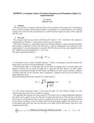
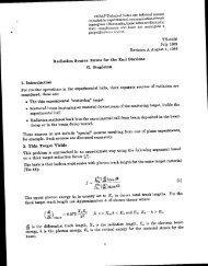
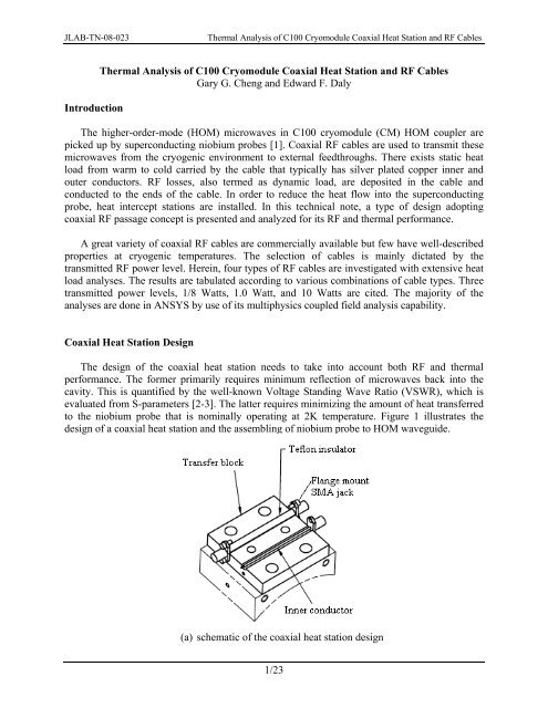
JLAB-TN-08-023Thermal Analysis of C100 Cryomodule Coaxial Heat Station and RF CablesIntroductionThermal Analysis of C100 Cryomodule Coaxial Heat Station and RF CablesGary G. Cheng and Edward F. DalyThe higher-order-mode (HOM) microwaves in C100 cryomodule (CM) HOM coupler arepicked up by superconducting niobium probes [1]. Coaxial RF cables are used to transmit thesemicrowaves from the cryogenic environment to external feedthroughs. There exists static heatload from warm to cold carried by the cable that typically has silver plated copper inner andouter conductors. RF losses, also termed as dynamic load, are deposited in the cable andconducted to the ends of the cable. In order to reduce the heat flow into the superconductingprobe, heat intercept stations are installed. In this technical note, a type of design adoptingcoaxial RF passage concept is presented and analyzed for its RF and thermal performance.A great variety of coaxial RF cables are commercially available but few have well-describedproperties at cryogenic temperatures. The selection of cables is mainly dictated by thetransmitted RF power level. Herein, four types of RF cables are investigated with extensive heatload analyses. The results are tabulated according to various combinations of cable types. Threetransmitted power levels, 1/8 Watts, 1.0 Watt, and 10 Watts are cited. The majority of theanalyses are done in ANSYS by use of its multiphysics coupled field analysis capability.Coaxial Heat Station DesignThe design of the coaxial heat station needs to take into account both RF and thermalperformance. The former primarily requires minimum reflection of microwaves back into thecavity. This is quantified by the well-known Voltage Standing Wave Ratio (VSWR), which isevaluated from S-parameters [2-3]. The latter requires minimizing the amount of heat transferredto the niobium probe that is nominally operating at 2K temperature. Figure 1 illustrates thedesign of a coaxial heat station and the assembling of niobium probe to HOM waveguide.(a) schematic of the coaxial heat station design1/23

JLAB-TN-08-023Thermal Analysis of C100 Cryomodule Coaxial Heat Station and RF Cables(b) Niobium probe assembled to HOM waveguideFig. 1 Coaxial heat station and niobium probeThe coaxial heat station has dual channels. There are a total of four flange mount SMA jacksfacilitating the connection of RF cables with SMA terminations. The basic idea of this design isto construct the simplest shape of RF path, a coaxial transmission line, and try to conduct theheat out of the inner conductor radially through the insulator. The transfer block is made ofoxygen-free high conductivity copper (OFHC), which has very good thermal conductivity atcryogenic temperatures. The inner conductor is made of 99.99% pure copper that has excellentthermal conductivity. The insulator is made of Teflon PTFE, which has low thermalconductivities from room temperature to cryogenic temperature. The reasons for using Teflon,not Sapphire or Alumina, include that it allows smooth impedance match between the heatstation and the flange mount SMA jacks, which also have Teflon PTFE insulators, and Teflon iscomparatively more cost-effective to be built into the heat station.It is noticed that Teflon PTFE experiences a noticeable thermal contraction when it is cooledfrom room temperature to 4K. According to a reliable data source [4], at 4K the thermalcontraction strain of Teflon PTFE is ε PTFE = (L 4K -L 293K )/L 293K = -0.021. For OFHC [5], thecontraction strain is ε OFHC = (L 4K -L 293K )/L 293K = -0.00326. That means the PTFE will shrink 6~7times more than OFHC does. This phenomenon may induce delamination between the OFHCand Teflon so that the thermal conduction path is interrupted. To avoid this, the Teflon is precompressedto an estimated amount during room temperature assembling. Also, Belleville springwashers are used to maintain clamping force when the heat station is cold.The coaxial heat station can be mounted on return headers and be convectively cooled. Or,it can be bolted to the 50K thermal shield to be conductively cooled. The 50K thermal shield hasactive cooling. Thus, both mounting methods are convectively cooled eventually. The bolt holeson the station make it convenient to install while maintaining the required clamping force to keepTeflon in thermal contact with the OFHC holder.2/23

JLAB-TN-08-023Thermal Analysis of C100 Cryomodule Coaxial Heat Station and RF CablesHeat Station and RF Cable Thermal AnalysisEvaluation of RF Losses in Coaxial CablesThere are two types of RF losses in a coaxial cable: surface loss and dielectric loss. The latteris omitted in all subsequent thermal analysis since it is small. Given the incipient RF power andnecessary coax dimensions and surface material resistivity, the surface loss can be calculated byclassic formulas. Appendix A presents the appropriate formulas and the derivation procedure, aswell as some usage notes.The vendors of RF cables usually provide calculation formulas for RF loss in decibels. Bydefinition, the loss DB isTherefore, the RF power loss down the cable is:⎛ Poutput⎞los _ db = 10log ⎜ ⎟10(1)⎝ Pinput⎠los _ db⎛ − ⎞= − = ⎜ −10P ⎟losPinputPoutputPinput1 10(2)⎜⎟⎝⎠Note that the los_db is normally negative, however, the vendors may give the absolute value ofthe los_db. That is the reason for the minus sign and absolute operator in Eq. (2). The RF losscalculated by Eq. (2) include surface loss and dielectric loss in the cable.A comparison of the room temperature RF losses calculated by the vendor’s and classicformulas for four example cables is given in Appendix B. The loss data for an illustrative casefeatured with incipient power = 10 W, cable length = 6 feet, frequency = 2.8 GHz, andimpedance = 50 Ω, are listed in Table 1. It is seen that the losses by classic formula may deviateas much as 13% from those calculated from the vendor’s formula. More comparisons are madein Appendix B. The classic formulas explicitly include the resistance/resistivity term that is afunction of temperature. Whereas the vendor’s loss dB formulas are for room temperaturecondition, they can be approximately scaled by square root of resistivity ratio to attain the lossdB at cryogenic temperatures. In the analyses that followed, the classic RF loss formulas areemployed.Table 1 RF losses in 6-foot cable at room temperatureInner Loss dB per RF loss per vendor’s RF loss per classicCable typeconductor OD vendor’s formula dB, P l vendor , Watts formula, P l , WattsGore type 89 0.02" 2.002 3.694 4.118Gore type 27 0.028" 1.459 2.853 2.912TFlex-402 0.036" 1.249 2.5 2.175Gore type 41 0.054" 0.777 1.638 1.5223/23

JLAB-TN-08-023Thermal Analysis of C100 Cryomodule Coaxial Heat Station and RF CablesSpecifications for Sample Coaxial RF CablesGore type 89 cableInner conductor material Silver plated copper 40 microinches minimum platingInsulator material ePTFE ε r = 1.4Outer conductor material Silver plated copper 40 microinches minimum platingBraided wire shield material Silver plated copper 40 microinches minimum platingInner conductor OD 0.02 InchesOuter conductor ID 0.055 InchesOuter conductor OD 0.062 InchesBraided wire diameter 0.00314 Inches = (40 Gauge)Braided wire strands # 80Gore type 27 cableInner conductor material Silver plated copper 40 microinches minimum platingInsulator material ePTFE ε r = 1.4Outer conductor material Silver plated copper 40 microinches minimum platingBraided wire shield material Silver plated copper 40 microinches minimum platingInner conductor OD 0.028 InchesOuter conductor ID 0.078 InchesOuter conductor OD 0.086 InchesBraided wire diameter 0.004 InchesBraided wire strands # 112Gore type 41 cableInner conductor material Silver plated copper 40 microinches minimum platingInsulator material ePTFE ε r = 1.4Outer conductor material Silver plated copper 40 microinches minimum platingBraided wire shield material Silver plated copper 40 microinches minimum platingInner conductor OD 0.054 inchesOuter conductor ID 0.146 InchesOuter conductor OD 0.154 InchesBraided wire diameter 0.004 InchesBraided wire strands # 1444/23

JLAB-TN-08-023Thermal Analysis of C100 Cryomodule Coaxial Heat Station and RF CablesTimes Microwave TFlex-402 cableInner conductor material Silver plated copper 40 microinches minimum platingInsulator material PTFE ε r = 2.04Outer conductor material Silver plated copper 40 microinches minimum platingBraided wire shield material Silver plated copper 40 microinches minimum platingInner conductor OD 0.036 InchesOuter conductor ID 0.118 InchesOuter conductor OD 0.128 InchesBraided wire diameter 0.00314 Inches = (40 Gauge)Braided wire strands # 160Thermal Performance of Double Heat Stations DesignFigure 2 illustrates the double heat station design. Note that only half of the dual-channelmodel is built due to symmetry.Fig. 2 Layout of the double heat station design5/23

JLAB-TN-08-023Thermal Analysis of C100 Cryomodule Coaxial Heat Station and RF CablesA 6-foot coaxial cable is used to connect the warm boundary (300K) to a nominal 50Kcoaxial heat station. The bottom surface of the 50K heat station will be conductively cooled bythe 50K thermal shield. Then a 2-foot coaxial cable connects the 50K heat station to a nominal5K coaxial heat station, which is bolted to liquid helium (LHe) headers or liquid level assemblypipes for convective cooling. There is another 2-foot coaxial cable connecting the 5K heat stationto the 2K niobium probe on HOM coupler. Cut-out views of the 5K and 50K station models areshown in Figs. 3 and 4. Figure 5 [6] shows a coaxial heat station connected with TFlex 402 RFcables.Fig. 3 50K coaxial heat station cut-out6/23

JLAB-TN-08-023Thermal Analysis of C100 Cryomodule Coaxial Heat Station and RF CablesFig. 4 5K coaxial heat station cut-outFig. 5 Coaxial heat station with single channel connected7/23

JLAB-TN-08-023Thermal Analysis of C100 Cryomodule Coaxial Heat Station and RF CablesVarious cabling schemes are analyzed for the corresponding heat loads dissipated to the 2Kniobium probe, LHe, 50K thermal shield, and 300K warm boundary. Three transmitted RFpower levels are considered: 10 Watts, 1.0 Watt, and 0.125 Watts. The static, dynamic, andensemble heat loads are presented in Tables 2, 3, and 4. For example, the “41-27-27” stands forone 6-foot Gore type 41 cable and two 2-foot Gore type 27 cables to complete the connection.The peak temperature is found to occur in the 6 feet cable connecting warm boundary to the 50Kcoaxial heat station. The peak temperatures are listed in Table 3 to help in judging whether theselected cables are safe from overheating and damage. The PTFE Teflon insulator will enter intoa gel status at 327 o C (600 K). Risky connections are red or yellow shaded in Table 4.Table 2 Double coaxial station design static loadsConnectionqs_2K,mWqs_LHe,mWqs_50K,mWqs_300K,mW41-27-27 0.95 128.8 87.26 -217402-89-89 0.39 77.4 79.92 -157.741-41-41 1.72 176.2 38.86 -216.8402-402-402 1.33 155.5 0.99 -157.827-27-27 0.95 129.1 -13.25 -116.889-89-89 0.40 77.9 -16.94 -61.3Table 3 Double coaxial heat station design dynamic loadsConnectionTransmittedpower, Wattsqd_2K,mWqd_LHe,mWqd_50K,mWqd_300K,mW41-27-27 10 341.6 597.3 1,097 806.141-27-27 1 5.74 9.44 61.31 71.5941-27-27 0.125 0.73 1.24 7.73 7.71402-89-89 10 546.3 1,002 1,627 1,137402-89-89 1 7.49 14.48 98.55 110.2402-89-89 0.125 0.92 2.92 7.23 8.8741-41-41 10 35.89 73.57 779.5 806.241-41-41 1 3.52 4.88 56.2 71.7141-41-41 0.125 0.44 0.7 7.18 7.71402-402-402 10 50.13 199.9 1,278 1,133402-402-402 1 4.59 7.03 89.44 110.1402-402-402 0.125 0.58 0.97 7.55 13.5927-27-27 1 5.74 9.11 130.3 147.227-27-27 0.125 0.72 1.57 13.94 14.1189-89-89 1 7.37 14.43 199.5 206.889-89-89 0.125 0.92 2.8 18.68 23.028/23

JLAB-TN-08-023Thermal Analysis of C100 Cryomodule Coaxial Heat Station and RF CablesTable 4 Double coaxial station design total heat loads and peak temperaturesConnectionTransmittedpower, Wattsq_2K,mWq_LHe,mWq_50K,mWq_300K,mWT_max,K41-27-27 10 342.55 726.10 1184.26 589.10 67141-27-27 1 6.69 138.24 148.57 -145.41 30041-27-27 0.125 1.67 130.04 94.99 -209.29 300402-89-89 10 546.69 1079.39 1706.92 979.30 1728402-89-89 1 7.88 91.87 178.47 -47.50 349402-89-89 0.125 1.31 80.31 87.15 -148.83 30041-41-41 10 37.61 249.77 818.36 589.40 67241-41-41 1 5.24 181.08 95.06 -145.09 30041-41-41 0.125 2.16 176.90 46.04 -209.09 300402-402-402 10 51.46 355.40 1278.99 975.20 1722402-402-402 1 5.92 162.53 90.43 -47.70 350402-402-402 0.125 1.91 156.47 8.55 -144.21 30027-27-27 1 6.69 138.21 117.05 30.40 50427-27-27 0.125 1.67 130.67 0.69 -102.69 30089-89-89 1 7.76 92.29 182.56 145.48 104489-89-89 0.125 1.32 80.66 1.74 -38.30 310Thermal Performance of Single Heat Station DesignA simpler design is to replace the 50K coaxial heat station with a thermal clamp, see Fig. 6.Figure 7 [6] shows a 50K clamp installed on test vehicle. The 50K clamp is made of OFHC andclamped over the FEP outer sleeve of coaxial cable. Sometimes, to enhance the cooling of thecable outer conductor, the FEP shield is stripped off. In simulations conducted hereafter, FEPshield is assumed to be intact. FEP has a low thermal conductivity of 0.195 W/m-K. This is asimpler design and hence more economical.The static, dynamic, and total heat loads are presented in Tables 5, 6, and 7. For example,“41-5K-27” means that one 8-feet Gore type 41 cable is heat sunk with a 50K clamp andconnects to a nominal 5K coaxial heat station, which is linked to the niobium probe by a 2- feetGore type 27 cable. Comparing to the double coaxial heat stations design, the single coaxial heatstation design yields higher heat loads to the 2K probe, 50K shield, and LHe cooling fluid.9/23

JLAB-TN-08-023Thermal Analysis of C100 Cryomodule Coaxial Heat Station and RF CablesFig. 6 Single coaxial heat station configuration50K clampFig. 7 50K clamp for RF cables10/23

JLAB-TN-08-023Thermal Analysis of C100 Cryomodule Coaxial Heat Station and RF CablesTable 5 Single coaxial station design static loadsConnectionqs_2K,mWqs_LHe,mWqs_50K,mWqs_300K,mW41-5K-27 1.23 141.3 396.80 -539.3402-5K-89 0.53 96.8 332.30 -429.641-5K-41 1.76 140.8 396.80 -539.3402-5K-402 1.01 96.4 332.30 -429.627-5K-27 0.63 70.6 252.30 -323.489-5K-89 0.25 38.5 128.70 -167.4Table 6 Single coaxial station design dynamic loadsTransmittedConnectionpower,Wattsqd_2K,mWqd_LHe,mWqd_50K,mWqd_300K,mW41-5K-27 10 372.30 986.40 121.20 817.3041-5K-27 1 6.25 46.14 9.99 77.3141-5K-27 0.125 0.77 4.61 1.18 8.74402-5K-89 10 577.10 1608.00 166.70 1181.00402-5K-89 1 8.01 89.84 13.25 121.20402-5K-89 0.125 0.97 6.69 1.42 12.4741-5K-41 10 43.67 698.60 120.30 817.2041-5K-41 1 4.14 44.04 9.98 77.3141-5K-41 0.125 0.51 4.35 1.17 8.74402-5K-402 10 61.17 1108.00 165.20 1181.00402-5K-402 1 5.64 86.27 13.24 121.20402-5K-402 0.125 0.67 6.25 1.42 12.4727-5K-27 1 0.71 126.60 18.76 155.8027-5K-27 0.125 0.83 8.72 2.02 16.4589-5K-89 1 8.65 194.40 24.62 214.1089-5K-89 0.125 1.06 16.38 2.75 25.6311/23

JLAB-TN-08-023Thermal Analysis of C100 Cryomodule Coaxial Heat Station and RF CablesTable 7 Double coaxial station design total heat loads and peak temperaturesConnectionTransmittedpower, Wattsq_2K,mWq_LHe,mWq_50K,mWq_300K,mWT_max,K41-5K-27 10 373.53 1127.70 518.00 278.00 94941-5K-27 1 7.48 187.44 406.79 -461.99 30041-5K-27 0.125 2.00 145.91 397.98 -530.57 300402-5K-89 10 577.63 1704.84 499.00 751.40 2676402-5K-89 1 8.54 186.68 345.55 -308.40 421402-5K-89 0.125 1.50 103.53 333.72 -417.13 30041-5K-41 10 45.43 839.40 517.10 277.90 94941-5K-41 1 5.90 184.84 406.78 -461.99 30041-5K-41 0.125 2.27 145.15 397.97 -530.57 300402-5K-402 10 62.18 1204.36 497.50 751.40 2675402-5K-402 1 6.64 182.63 345.54 -308.40 421402-5K-402 0.125 1.68 102.61 333.72 -417.13 30027-5K-27 1 1.34 197.15 271.06 -167.60 69227-5K-27 0.125 1.46 79.27 254.32 -306.95 30089-5K-89 1 8.90 232.86 153.32 46.70 158789-5K-89 0.125 1.31 54.84 131.45 -141.77 334Thermal Performance of No Coaxial Heat Station DesignFor low RF power applications, a straight coaxial cable that is heat sunk by a 50K clampcould be a simple and economical design option for transmitting the HOM signal to outside. Thestatic, dynamic, and total heat loads to the 2K niobium probe, 50K thermal shield, and 300Kwarm boundary are analyzed for the mentioned four types of coaxial cables. The results arepresented in Tables 8, 9, and 10 for information. For example, the connection “41-41” means anominal 8-feet Gore type 41 cable is used between 2K probe and the external feedthrough. Thecable is heat sunk to 50K thermal shield by use of a clamp. By comparing the total heat transferto 2K probe in all design options for same type of cable cases, it is easy to find that no coaxialheat station design has much more heat dumped to 2K. The ratios range from 18 to 147.Table 8 No coaxial heat station design static loadTransmittedConnectionpower,Wattsqs_2K,mWqs_50K,mWqs_300K,mW41-41 10, 1, 0.125 182.90 384.20 -567.1402-402 10, 1, 0.125 113.50 324.30 -437.727-27 1, 0.125 79.98 247.50 -327.589-89 1, 0.125 41.44 127.30 -168.712/23

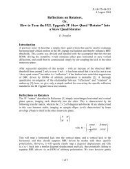
JLAB-TN-08-023Thermal Analysis of C100 Cryomodule Coaxial Heat Station and RF CablesTable 9 No coaxial heat station design dynamic loadTransmittedConnectionpower,Wattsqd_2K,mWqd_50K,mWqd_300K,mW41-41 10 648.10 76.95 772.0041-41 1 31.32 7.36 60.7841-41 0.125 3.33 0.92 6.97402-402 10 1069.00 97.83 1151.00402-402 1 72.10 9.12 108.70402-402 0.125 5.18 1.13 10.5727-27 1 117.40 13.87 147.6027-27 0.125 7.34 1.71 14.4389-89 1 187.20 20.13 209.1089-89 0.125 14.07 2.44 23.58Table 10 No coaxial heat station design total heat loadTransmittedConnectionpower,Wattsq_2K,mWq_50K,mWq_300K,mWT_max,K41-41 10 831.00 461.15 204.90 81841-41 1 214.22 391.56 -506.32 30041-41 0.125 186.23 385.12 -560.13 300402-402 10 1182.50 422.13 713.30 2511402-402 1 185.60 333.42 -329.00 365402-402 0.125 118.68 325.43 -427.13 30027-27 1 197.38 261.37 -179.90 61727-27 0.125 87.32 249.21 -313.07 30089-89 1 228.64 147.43 40.40 150089-89 0.125 55.51 129.74 -145.12 317Comparison of HOM RF Passages in Horizontal Test Bed (HTB)Figure 8 shows a view of the HTB test module that contains two cavities. The test setupincluded three types of HOM signal passages: 1) microwave path contains one SMA femalefemalebullet and two coaxial RF cables, 2) path contains one coaxial heat station and twoconnecting cables, and 3) path made of one coaxial RF cable. Figure 9 shows the RF cablingdetails [6] in the HTB test module. The 50K cable clamp is positioned at approximately 2-feetfrom the tophat end.Test results show that the connection using one coaxial heat station yields the lowesttemperature at 2K probe. That indicates the coaxial heat station is effective in removing the RFheating in HOM microwave transmission. Nevertheless, the C100 CM adopts no coaxial heatstation design notion, using TFlex 402 cable, since the observed temperature at 2K probe is13/23

JLAB-TN-08-023Thermal Analysis of C100 Cryomodule Coaxial Heat Station and RF Cablesacceptable. This implies that the HOM RF power may not be so high. It is estimated that theaverage HOM power is around 0.125W.Fig. 8 HTB test moduleNote that in the simulation, a 2K temperature boundary has been set at the cold end of thecable for all cases. This is not exactly true in reality since when the heat transfer to 2K probe willraise the temperature to be above 2K. The final temperature of the probe is up to thermalequilibrium that is reached. The model did not intend to include all parts from top to toe. Theheat numbers presented in previous tables are good to be used as reference and the basis ofcomparison between different designs.14/23

JLAB-TN-08-023 Thermal Analysis of C100 Cryomodule Coaxial Heat Station and RF CablesFig. 9 HTB RF cabling schemes15/23

JLAB-TN-08-023Thermal Analysis of C100 Cryomodule Coaxial Heat Station and RF CablesSummaryCoaxial heat station used to transmit C100 Cryomodule HOM signal is developed. Thethermal performance of such heat station is evaluated for three types of design: 1) the doublecoaxial heat station design, 2) the single coaxial heat station design, and 3) no coaxial heatstation design. An apparent judgement is confirmed that the more coaxial heat stations used, thenthe lower the heat being transferred to 2K probe. The coaxial heat station certainly increasessystem complexity and cost. Since the HTB test of two C100 CM cavities indicates a simpleconnection without any coaxial station could lead to satisfactory thermal performance, C100 CMadopts the no coaxial heat station design. The coaxial heat station is helpful if the HOM RFpower is high, for example, higher than 1 Watt. Among the connections that have been analyzed,no safe cabling scheme is found for the RF power level of 10 Watts.REFERENCES[1]. C. E. Reece, E. F. Daly, T. Elliott, H. L. Phillips, J. P. Ozelis, T. Rothgeb, K. Wilson, andG. Wu, “High Thermal Conductivity Cryogenic RF Feedthroughs for Higher Order ModeCouplers,” in Proceedings of 2005 Particle Accelerator Conference, Knoxville, TN, 2005, pp.4108-4110.[2]. D. M. Pozar, “Microwave Engineering,” Addison-Wesley Publishing Company, Inc.,1990.[3]. S. Ramo, J. R. Whinnery, T. V. Duzer, “Fields and Waves in CommunicationElectronics,” John Wiley & Sons, Inc., 1993.[4]. http://cryogenics.nist.gov/MPropsMAY/Teflon/Teflon_rev.htm[5]. J. E. Jensen, W. A. Tuttle, R. B. Stewart, H. Brechna, and A. G. Prodell, “BrookhavenNational Laboratory Selected Cryogenic Data Notebook,” Brookhaven National LaboratoryAssociated Universities, Inc., Revised August 1980.[6]. Provided by L. King, Jefferson Lab.16/23

JLAB-TN-08-023Thermal Analysis of C100 Cryomodule Coaxial Heat Station and RF CablesAPPENDICESA. Formulation of RF Surface Loss in Coaxial CablesNomenclature:a ----- Outer radius of inner conductor δ ----- Skin depthb ----- Inner radius of outer conductor ε ----- PermittivityA ----- Area η ----- Constant impedanceD ----- Diameter µ ----- PermeabilityI ----- Surface current ρ ----- ResistivityL ----- Cable length i ----- Subscript for “inner”P ----- Power o ----- Subscript for “outer” or “null”Z ----- Impedance r ----- Subscript for “relative”s ----- Subscript for “surface”A.1 Surface Loss per Unit Area Expressed with Surface CurrentThe general form of the electrical resistance in skin depth can be expressed asρ L ρ L LR = = = R sAδπ Dδπ Dρwhere the surface resistance, Rs=δ, is temperature dependent.For the inner and outer conductors respectively,LLRi = R sRo= Rs2π a2π bP2 inputThe surface current square is evaluated as:I =ZThe power deposition onto inner and outer conductors can be expressed as:2 2 L2 2 LPi= I Ri= I RsPo= I Ro= I Rs2π a2π bThus, the RF losss per unit area (W/m 2 ) is:PiI R=2πa L 4πa2s2 2PiI R=2πb L 4πb2s2 2A.2 Surface Loss per Unit Volume Expressed with Surface CurrentSometimes it is necessary to know the power deposition per unit volume (W/m 3 ):17/23

JLAB-TN-08-023Thermal Analysis of C100 Cryomodule Coaxial Heat Station and RF CablesP I Lπ a L 2π aP I Lπ b L 2π b22io= R2 s= R2 sA.3 Surface Loss per Unit Area Expressed with Transmitted PowerThe impedance in a coax is defined as [3]:Zlnbaπμεlnbaπμr oo= == η and η = = 376. 6Ω22εrμεolnbaπ21εrμεoThe surface current square can be expresses in terms of input power as:Pinput2πP2inputI = =Z bη lnaThen the power depositions to inner and outer conductors are:PinputLP22input LPiI Ri= RsPo= I Ro= Rb ab bη lnη lnaaThus, the RF losss per unit area (W/m 2 ) is:=sP P εi12πa L b 2πaη lnaP P ε 12πb L b 2πbη lnainput ro input r= Rs= R2s 2B. Comparison of RF Losses in Cables by Classic and Vendor’s FormulasP input:= 10⋅Wf := 2.8 × 10 9 ⋅HzL o := 6ft ⋅ Z o := 50⋅ohm μ o 4⋅π⋅10 − 7 H:= ⋅ ε o 8.854 10 − 12 F:= ⋅ ⋅mm1. Type 89 Gore coax cable having silver-plated copper conductors:0.02a := ⋅in ε ePTFE := 1.42ε ePTFE ⋅ε o2⋅π⋅Z o ⋅μ ob := a⋅eb = 0.027inRF loss by vendor's formula:18/23

JLAB-TN-08-023Thermal Analysis of C100 Cryomodule Coaxial Heat Station and RF CablesfLos_db ( x) := 0.02 + 0.004⋅+ 0.01⋅Los_db ( L o ) = 2.00210 9 ⋅Hzf10 9 ⋅Hz+x12⋅in⎛⎜⎝⋅f−0.00251+ 0.00412⋅+ 0.18925⋅10 9 ⋅Hzf10 9 ⋅Hz⎞⎟⎠⎛⎜−Los_db()x10P l_vendor () x := P input ⋅⎝1 − 10 ⎠ P l_vendor L o⎞⎟( ) = 3.694WRF loss by classic formula:Room temperature silver resistivity from www.matweb.comρ_Ag 1.55⋅10 8P input:= ⋅ohm⋅mRs := π⋅f⋅μ o ⋅ρ_AgRs = 0.013Ω I sq :=Z oxE.R. in inner conductor skin depth: R i () x := ⋅Rs2π⋅aR i ( L o ) = 15ΩxE.R. in outer conductor skin depth: R o () x := ⋅Rs2π⋅bR o ( L o ) = 5.592ΩTotal RF surface loss:P l () x := I sq ⋅( R o () x + R i () x ) P l L o =A plot of RF power loss in cable of length 1.0' to 6.0' is shown as follows:( ) 4.118W4P l_vendor ( x)P l () x21 2 3 4 5 6x12⋅inA plot of RF power loss in type 89 cable of length 2' to 50' is shown in the next page. It isnoticed that the classic formulas will generate erroneous RF power loss when the cable lengthexceeds 15 feet approximately. Care must be taken when using the classic formulas on long RFcables.19/23

JLAB-TN-08-023 Thermal Analysis of C100 Cryomodule Coaxial Heat Station and RF Cables20/23

JLAB-TN-08-023Thermal Analysis of C100 Cryomodule Coaxial Heat Station and RF Cables2. Type 41 Gore coax cable having silver-plated copper conductors:0.0540.146a := ⋅in b := ⋅in22b = 0.073inRF loss by vendor's formula:fLos_db ( x) := 0.02468+ 0.01052⋅+ ( −0.01148)⋅Los_db ( L o ) = 0.777⎛10 9 ⋅Hzf+10 9 ⋅Hz− Los_db()x⎜10 ⎟P l_vendor () x := P input ⋅⎝1 − 10 ⎠ P l_vendor L o⎞x⋅12⋅in⎛⎜⎝( ) = 1.638W0.00077+ 0.00089⋅f+ 0.07194⋅10 9 ⋅Hzf10 9 ⋅Hz⎞⎟⎠RF loss by classic formula:Rs :=R i () xπ⋅f⋅μ o ⋅ρ_Agx:= ⋅Rs R i L o2π⋅aTotal RF surface loss:P inputRs = 0.013Ω I sq :=Z ox= R o () x := ⋅Rs R o L o2π⋅b( ) 5.555Ω⋅( )P l () x := I sq R o () x + R i () x P l L o( ) = 1.522W( ) = 2.055ΩA plot of RF power loss in cable of length 1.0' to 6.0' is shown below:4P l_vendor ( x)P l ( x)21 2 3 4 5 6x12⋅in21/23

JLAB-TN-08-023Thermal Analysis of C100 Cryomodule Coaxial Heat Station and RF Cables3. Type 27 Gore coax cable having silver-plated copper conductors:0.0280.078a := ⋅in b := ⋅in22b = 0.039inRF loss by vendor's formula:fLos_db ( x) := 0.02314+ 0.00904⋅+ ( −0.01663)⋅Los_db ( L o ) = 1.459⎛10 9 ⋅Hzf+10 9 ⋅Hz− Los_db()x⎜10 ⎟P l_vendor () x := P input ⋅⎝1 − 10 ⎠ P l_vendor L o⎞x⋅12⋅in⎛⎜⎝( ) = 2.853W0.00353+ 0.00270⋅f+ 0.13664⋅10 9 ⋅Hzf10 9 ⋅Hz⎞⎟⎠RF loss by classic formula:Rs := π⋅f⋅μ o ⋅ρ_AgRs = 0.013ΩP inputxI sq := R i () x := ⋅Rs R i L oZ o2π⋅aTotal RF surface loss:⋅( )P l () x := I sq R o () x + R i () x P l L o( ) = 2.912Wx= R o () x := ⋅Rs R o L o2π⋅b( ) 10.714ΩA plot of RF power loss in cable of length 1.0' to 6.0' is shown below:3( ) = 3.846ΩP l_vendor ( x)2P l ( x)11 2 3 4 5x12⋅in622/23

JLAB-TN-08-023Thermal Analysis of C100 Cryomodule Coaxial Heat Station and RF Cables4. TFlex-402 semirigid coax cable having silver-plated copper conductors:0.0360.118a := ⋅in b := ⋅in22Check the impedance in cable:ln⎛b ⎞⎜⎝ a ⎟⎠ μ oZ :=2π⋅ε PTFE ⋅ε ob= 0.059in ε PTFE := 2.04Z = 49.837ΩRF loss by vendor's formula:⎛ff xLos_db ( x) :=⎜0.33⋅ 10 6 + 0.00120⋅⎝ ⋅Hz10 6 ⎟⋅Los_db L o100⋅ft⋅Hz⎠⎛ − Los_db()x ⎞⎜10 ⎟P l_vendor () x := P input ⋅⎝1 − 10 ⎠ P l_vendor L o =RF loss by classic formula:⎞( ) 2.5WP inputRs := π⋅f⋅μ o ⋅ρ_AgRs = 0.013Ω I sq :=Z oxxR i () x := ⋅Rs R i ( L o ) = 8.333Ω R o () x := ⋅Rs R o L o2π⋅a2π⋅b( ) = 1.249( ) = 2.542ΩTotal RF surface loss:⋅( )P l () x := I sq R o () x + R i () xP l ( L o ) = 2.175WA plot of RF power loss in cable of length 1.0' to 6.0' is shown below:3P l_vendor ( x)2P l ( x)11 2 3 4 5x12⋅in623/23