Magnetic Field Induced Semimetal-to-Canted-Antiferromagnet ...

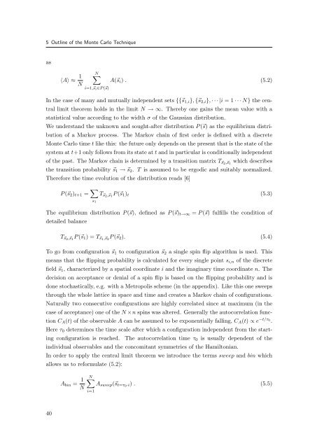
5 Outline of the Monte Carlo Technique
as
〈A〉 ≈ 1
N
N�
i=1,�si∈P (�s)
A(�si) . (5.2)
In the case of many and mutually independent sets {{�s1,i}, {�s2,i}, · · · |i = 1 · · · N} the cen-
tral limit theorem holds in the limit N → ∞. Thereby one gains the mean value with a
statistical value according to the width σ of the Gaussian distribution.
We understand the unknown and sought-after distribution P (�s) as the equilibrium distri-
bution of a Markov process. The Markov chain of first order is defined with a discrete
Monte Carlo time t like this: the future only depends on the present that is the state of the
system at t+1 only follows from its state at t and in particular is conditionally independent
of the past. The Markov chain is determined by a transition matrix T�s2,�s1 which describes
the transition probability �s1 → �s2. T is assumed to be ergodic and suitably normalized.
Therefore the time evolution of the distribution reads [6]
P (�s2)t+1 = �
s1
T�s2,�s1 P (�s1)t
(5.3)
The equilibrium distribution P (�s), defined as P (�s)t→∞ = P (�s) fulfills the condition of
detailed balance
T�s2,�s1 P (�s1) = T�s1,�s2 P (�s2). (5.4)
To go from configuration �s1 to configuration �s2 a single spin flip algorithm is used. This
means that the flipping probability is calculated for every single point si,n of the discrete
field �s1, characterized by a spatial coordinate i and the imaginary time coordinate n. The
decision on acceptance or denial of a spin flip is based on the flipping probability and is
done stochastically, e.g. with a Metropolis scheme (in the appendix). Like this one sweeps
through the whole lattice in space and time and creates a Markov chain of configurations.
Naturally two consecutive configurations are highly correlated since at maximum (in the
case of acceptance) one of the N ×n spins was altered. Generally the autocorrelation func-
tion CA(t) of the observable A can be assumed to be exponentially falling, CA(t) ∝ e −t/τ0 .
Here τ0 determines the time scale after which a configuration independent from the start-
ing configuration is reached. The autocorrelation time τ0 is usually dependent of the
individual observables and the concomitant symmetries of the Hamiltonian.
In order to apply the central limit theorem we introduce the terms sweep and bin which
allows us to reformulate (5.2):
40
Abin = 1
N
N�
Asweep(�st=τ0·i) . (5.5)
i=1