Magnetic Field Induced Semimetal-to-Canted-Antiferromagnet ...
Magnetic Field Induced Semimetal-to-Canted-Antiferromagnet ...
Magnetic Field Induced Semimetal-to-Canted-Antiferromagnet ...
You also want an ePaper? Increase the reach of your titles
YUMPU automatically turns print PDFs into web optimized ePapers that Google loves.
5 Outline of the Monte Carlo Technique<br />
time Green function is a projec<strong>to</strong>r,<br />
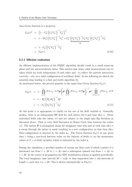
Gs(τ) 2 =<br />
�<br />
1 − U > �<br />
s<br />
= 1 − 2U > s<br />
= 1 − U > s<br />
U < s U > s<br />
�<br />
U < s U > s<br />
� −1<br />
U < s<br />
�<br />
U < s U > �−1 s U < s<br />
� 2<br />
� −1<br />
U < s + U > s<br />
�<br />
U < s U > s<br />
� −1<br />
U < s U > s<br />
� �� �<br />
=1<br />
�<br />
U < s U > �−1 s U < s<br />
= Gs(τ) . (5.16)<br />
5.2.1 Efficient realization<br />
An efficient implementation of the PQMC algorithm should result in a small warm-up<br />
phase and low au<strong>to</strong>correlation times. This assures that many valid measurements can be<br />
taken which are both independent of each other and - <strong>to</strong> reflect the particle interaction<br />
correctly - rely on a valid configuration of auxilliary fields. In the following we sketch the<br />
essential steps leading <strong>to</strong> a fast and stable algorithm [5].<br />
As mentioned before, the pivotal quantity is the equal time Green function Gs(τ),<br />
Gs(τ) = 1 −<br />
nτ �<br />
n=1<br />
= 1 − B > s<br />
= 1 − U > s<br />
e V(sn) e −∆τT P<br />
�<br />
B < s B > s<br />
�<br />
U < s U > s<br />
� −1<br />
B < s<br />
� −1<br />
U < s<br />
�<br />
P †<br />
m�<br />
n=1<br />
e V(sn) e −∆τT P<br />
� −1<br />
P †<br />
m�<br />
n=nτ +1<br />
e V(sn) e −∆τT<br />
(5.17)<br />
At this point it is appropriate <strong>to</strong> clarify on the use of the field variable s. Generally<br />
spoken, there is an independent HS field for each lattice site i and time slice n. Those<br />
individual fields take the values ±1 and are subject <strong>to</strong> the single spin flip decisions as<br />
discussed above. That is every field fluctuates in Monte Carlo time between the values<br />
±1. The matrix P is propagated along the imaginary time axis and at each time slice n<br />
a sweep through the lattice is made resulting in a new configuration on that time slice.<br />
This configuration is denoted by the index sn. The Green function Gs(τ) at any given<br />
time τ being a non-local function relies on the entirety of fields i.e on the momentary<br />
values of N × m field variables, which is indicated by the index s.<br />
During the simulation a specified number of sweeps are done each of which consists of a<br />
downward run from τ = 2θ <strong>to</strong> τ = ∆τ and a subsequent upward run from τ = ∆τ <strong>to</strong><br />
τ = 2θ. In the course of propagation the SDV stabilization scheme is applied periodically.<br />
The <strong>to</strong>tal imaginary time interval 2θ = m∆τ is thus segmented in<strong>to</strong> n sub-intervals of<br />
length τ1 such that nτ1 = 2θ. This is shown schematically in Fig.5.1.<br />
44


