Time Varying System Identification using Adaptive ... - IRNet Explore

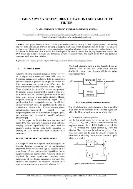
Time Varying System Identification using Adaptive FilterTIME VARYING SYSTEM IDENTIFICATION USING ADAPTIVEFILTERPANKAJ KUMAR PATHAK 1 , KANDARPA KUMAR SARMA 21,2 Department of Electronics and Communication Engineering, Gauhati University, Guwahati, Assam, IndiaE-mail id:pankaj0590@yahoo.co.in, kandarpaks@gmail.comAbstract—This paper presents a method of using an adaptive filter to identify a time varying systems. The primaryobjective is to formulate an approach of using an adaptive filter based system to identify systems. Some of the classicalapplications of adaptive filtering are system identification, channel equalization, signal enhancement, and prediction. Here,we discuss the formulation of an adaptive filter based system for identification of time varying properties of systems likeLCR circuit and simple pendulum. The formulated system successfully tracks the output of the LCR and pendulumresponses which show time variation.Keywords: Time varying systems, adaptive filtering, prediction, LCR circuit, Simple pendulum.I. INTRODUCTIONAdaptive filtering of signals is related to the recoveryof a signal from corrupted form with time orfrequency dependence. Adaptive filtering requires areference signal to produce an output for which thefilter parameters are adaptive modified and theresultant signal tracks the variations in the input.Thus, adaptation is, by itself a time-varying process.In general, signals encountered in practice may alsobe nonstationary, i.e., they change characteristics withtime (e.g., speech, music, radio signals). Hence,adaptive filtering of nonstationary signals is aproblem that deserves special attention. In addition,in many important cases, the problem can be seen asequivalent to identification of linear systems whoseoutput produces the desired signal. Asadaptive systems can track variations in input signal,this attribute can be used to identify unknownprocesses [1].In this paper, we have taken two examples andapplied the basic concepts of adaptive filter and timevarying systems. Specifically we have used anadaptive system trained with LMS algorithm toidentify an LCR circuit and track variations in apendulum.II. THEORETICAL CONSIDERATIONSAn adaptive filter is a system that self-adjusts itstransfer function according to an optimizationalgorithm driven by an error signal. Because of thecomplexity of the optimization algorithms, mostadaptive filters are digital filters. Adaptive filters arerequired for some applications because someparameters of the desired processing operation (forinstance, the locations of reflective surfaces in areverberant space) are not known in advance [2].The block diagram, shown in the figure1, shows anadaptive filter. It may use Least Mean Squares(LMS), Recursive Least Squares (RLS) and otherrelated algorithms.Fig.1: Adaptive filter with update algorithmThe idea behind the block diagram is that a variablefilter extracts an estimate of the desired signal forwhich the filter path gains are varied adaptively.A. Least mean square algorithmLet the tap input vector be given by x n = [x n (0),x n (1), ………x n (L-1)] T , which is convolved with theunknown system h n = [h n (0), h n (1)………….h n (L-1)] T to produce the signal sample y n. Now theadaptive filter output can be written as y/ n = x n * h n .This expression can be used to identify systems byadaptively minimizing the square of the error signalwhich is given by:e n = y n – y / nFigure2: System identification structure.IRNet Transactions on Electrical and Electronics Engineering (ITEEE) ISSN 2319 – 2577, Vol-1, Iss-2, 201249

Time Varying System Identification using Adaptive FilterB. RLS (Recursive least square)The updated equation of RLS algorithm is given as:h / n+1= h / n + k n e nwhere k n called kalman gain.C. AP(Affine projection) algorithmThe affine projection algorithm incorporates multipleprojections by concatenating past tap-input vectorsfrom time iteration n to time iteration (n-k+1), wherek is defined as projection order. To formulate the APalgorithm, we first define the sub selected and fulltap-input matrices [3].D. Time varying system model:Now,the above theories can be appled to identify theunkown systems.h n+1 = h n + (1- ) 1/2 s nwhere h n is the impulse response of the unknownsystem, and s n is a noise process[4]. Let us define aexpectation operator: E{h n }=0, E{w n }=0Misalignment vector which results in the error signal:v n = h / n -h nError signal: e n = w n – x T n v nNow; v n+1 = h / n+1-h n+1R v,n+1 = E{v n+1 v T n+1}= R v,n + 2(1- )ơ 2 Iwhere I is identity matrix and variance ơ 2 is 1,we canfind;E{v n v T n}=R v,nFrom the definition of the first-order Markov model:E{h n h T n}= E{s n s T n}=ơ 2 ISo, from the above calculation we can conlude thatthe adaptive filter is able to track the unknown systemand V nj is fluctuating around its mean so;E{V n-j V T n-j} ≠ E{S n S T n}= R vnwhere R vn is the autocorrelation matrix. LCR circuit output applied to the adaptivesystem: Let us consider a circuit shown infigure 3 having a capacitance C, inductanceL, and resistance R allare connected in series. When a constant emfis applied a momentary current flowsthrough it;E = q/C + L di/dt + iRputting i = dq/dt, we will get;d 2 q/dt 2 + 2k dq/dt + w 2 x = ...(1)Now, if we solve the differential equation (1) we willget the solution in the form;q 0 = q + [-q 0 /2(1 + k/(k 2 – w 2 ) 1/2 e {-k +(k2 – w2)1/2}t - q 0 /2(1 -k/(k 2 – w 2 ) 1/2 e {-k - (k2 – w2)1/2}t ] ...(2)Equation (2) shows the charge grows in LCR circuit,which depends on three cases;High damping when K 2 > w 2 , it shows thatcharge gradually reaches to final value. Critically damped when K 2 = w 2 . Critically damped when K 2 < w 2 .Now to check it weather it is time variant or not let usreplace it q(t) by q(t + ơ); where ơ is small change intime delay. If we put q(t) = q(t + ơ) we found q(t) ≠q(t + ơ) because of following reasons;(i) Equation (2) has terms which include L, C, R. ForL we know Ldi/dt, which shows current after sometime will definitely change because the circuit ischarging.(ii) For R we take in the form iR so it will alsochange and effect the whole equation.(iii) For C, we take q/C i.e it/C, so again current willchange with change in time because capacitor ischarging.So for all above parameters we get;Ldi/dt ≠ Ldi(t+ ơ)/dti(t)R ≠ i(t+ ơ)Rit/C ≠ i(t+ ơ)CIII. SYSTEM MODELThe system model is as in figure 3.Figure 4: Series LCR circuitwe can say charging and discharging of LCR circuitis a time varying system.Figure 3: System model using adaptive filterWe formulate an approach to apply the outputs of anLCR [5] circuit and a pendulum [6] to this system.Figure 5: Shows the damping conditions.IRNet Transactions on Electrical and Electronics Engineering (ITEEE) ISSN 2319 – 2577, Vol-1, Iss-2, 201250

Time Varying System Identification using Adaptive FilterNow let us try to shift the time axis of the abovegraph, but theoretically it is not possible to shift thetime axis either in positive side or negative sidebecause it is not possible to charge the circuit at timet= 2,3... directly, we need to start from 0. Alsopractically it is not possible to charge the circuit innegative time intervals which is not possiblepractically [7]. But still we try to analyze by using theconcept of shift variant and invariant. We shall applyimpulse function as given below;ơ(0) = 1But ơ (1) = 0ơ (-1)= 0So, for all these conditions we get only the stepresponse of the circuit as shown in figure 6 and thegraph will shift for this condition only which isalready discussed. Simple Pendulum : let us take anotherexample of simple pendulum containingsimple harmonic motion to find weather it istime variant or not.Let us consider a particle of mass ‘m’displacement ‘x’, and ‘F’ be the restoring force actingon the particle then the differential equation can bewritten asd 2 x/dt 2 + w 2 = 0 ...(3)Now, if we solve equation (3), we will get thesolution in the formX(t) = A sin (wt + Ø) ...(4)where;x(t) = displacement of the particle.A = maximum amplitude of the particle.w = angular velocity.Now, let us check equation (4) to find out whether itis time variant or not. Since we know that to satisfythe condition of SHM a particle must change itsamplitude which change its angle Ø, so it means thatthe term A sin (wt + Ø) will have some differentvalue as compared to Asin [w(t+ ơ) + Ø] whichgives;X(t) ≠ X(t+ ơ)Now, our aim is to apply adaptive filter to track andverify the above condition.Figure 6: Step response of LCR circuit for shift variantfunctionAfter that we take the output of LCR circuit andapply as an input of adaptive system with step size1.1, than we take MSE of the system to find thatweather our system is working properly or not, and itis observed that the error is not significant, which isshown in table 1.Table 1: MSE for LCR circuitCaseLCRcircuitTimein sec.1234567891011121314Output ofLCRcircuit(q).631.732.853.924.965.986.997.998.999.9910.9911.9912.9913.99Output ofadaptivesystem(q / ).661.812.994.125.216.287.348.399.4410.4911.5412.5913.6414.69MSE/q-q / / 2.48.42.35.30.24.20.15.12.08.06.03.02.0075.0009Figure 7: Phase angle tracking for simple pendulum.Table 2: Average MSE for LMS and RLSalgorithm.Algorithm Iterations Average MSELMSRLS51015510150.0080.0060.0040.0050.0030.002IRNet Transactions on Electrical and Electronics Engineering (ITEEE) ISSN 2319 – 2577, Vol-1, Iss-2, 201251

Time Varying System Identification using Adaptive FilterIV.CONCLUSIONWe see that with increase in number of trainingsessions, the MSE value steadily decreases. It meansthat the adaptive filter trained with LMS algorithm istracking the system properties. We repeat the abovewith RLS algorithm. The comparative results areshown in table 2.From table 1 and table 2, we see that an adaptivefilter trained with RLS tracks the time varyingcharacteristics of an LCR circuit and a Pendulum.REFERENCES[1] M. H. Hayes: Statistical Digital Signal and Modeling by JohnWiley and Sons.[2] J. Benesty and S. L. Gay: “An improved PNLMS algorithm,” inProc. IEEE Int. Conf. Acoust., Speech, Signal Process., 2002,vol. 2, pp. 1881–1884.[3] A. W. H. Khong and P. A. Naylor: “A family of selective-tapalgorithms for stereo acoustic echo cancellation,” in Proc.IEEE Int. Conf. Acoust., Speech, Signal Process., Mar. 2005.[4] P. A. Naylor and W. Sherliker: “A short-sort M-max NLMSpartial update adaptive filter with applications to echocancellation,” in Proc. IEEE Int. Conf. Acoust., Speech, SignalProcess., 2003, vol. 5.[5] Yu-Ching Lin and Ching-Hung Lee: System Identification andAdaptive Filter Using a Novel Fuzzy Neuro System,International journal of computational cognition, vol 5, No.1,March 2007.[6] M. Yukawa, K. Slavakis, and I. Yamada: “Adaptive parallelquadraticmetric projection algorithms,” IEEE Trans. SpeechAudio Process, vol. 15, no. 5, pp. 1665–1680, Jul. 2007.[7] M. Yukawa and I. Yamada: “Adaptive parallel variable-metricprojection algorithm—An application to acoustic echocancellation,” in Proc. IEEE ICASSP, Apr. 2007, pp. 1353–1356.[8] I. Yamada and N. Ogura: “Adaptive projected subgradientmethod for asymptotic minimization of sequence ofnonnegative convex functions,” Numer. Funct. Anal. Optim.,vol. 25, no. 7&8, pp. 593–617, 2004.[9] K. Slavakis, and K. Yamada: “An efficient robust adaptivefiltering algorithm based on parallel subgradient projectiontechniques,” IEEE Trans. Signal Processing, vol. 50, no. 5, pp.1091–1101, 2002IRNet Transactions on Electrical and Electronics Engineering (ITEEE) ISSN 2319 – 2577, Vol-1, Iss-2, 201252