Chapter 5 Methods of Images

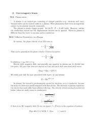
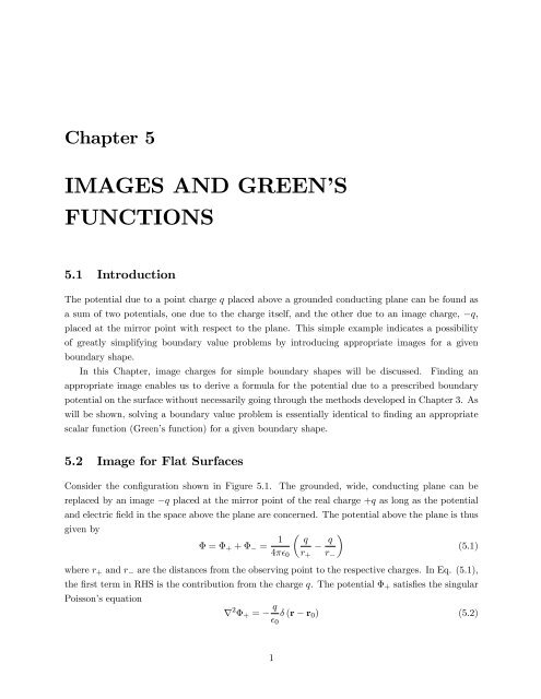
Chapter 5IMAGES AND GREEN’SFUNCTIONS5.1 IntroductionThe potential due to a point charge q placed above a grounded conducting plane can be found asa sum of two potentials, one due to the charge itself, and the other due to an image charge, q,placed at the mirror point with respect to the plane. This simple example indicates a possibilityof greatly simplifying boundary value problems by introducing appropriate images for a givenboundary shape.In this Chapter, image charges for simple boundary shapes will be discussed. Finding anappropriate image enables us to derive a formula for the potential due to a prescribed boundarypotential on the surface without necessarily going through the methods developed in Chapter 3. Aswill be shown, solving a boundary value problem is essentially identical to …nding an appropriatescalar function (Green’s function) for a given boundary shape.5.2 Image for Flat SurfacesConsider the con…guration shown in Figure 5.1.replaced by an imageThe grounded, wide, conducting plane can beq placed at the mirror point of the real charge +q as long as the potentialand electric …eld in the space above the plane are concerned. The potential above the plane is thusgiven by = + + = 14 0 qr +where r + and r are the distances from the observing point to the respective charges. In Eq. (5.1),the …rst term in RHS is the contribution from the charge q. The potential + satis…es the singularPoisson’s equationqr(5.1)r 2 + = q 0 (r r 0 ) (5.2)1

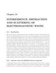
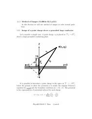
qr+Φconductor­qddr­image chargeFigure 5-1: Image charge for a ‡at conducting plate.where r 0 = de z is the location of the charge q. The image charge q is below the plane. Therefore,in the space above the plane, the potential due to the image charge should satisfy the Laplaceequaion without any singularities,r 2 = 0 (z > 0) (5.3)In other words, the potential can be regarded as a general solution to the singular Poisson’sequation in Eq. (5.2) which is added in order that the total potential satisfy the boundary condition, = 0 on the plane (5.4)Obviously, the solution + is the particular solution to the Poisson’s equation. Note that we have afreedom to add general solutions satisfying the Laplace equation to a particular solution satisfyingthe Poisson’s equation.Images for a grounded wedge can be similarly found. For example, if the wedge angle is 90 ,three images appear as shown in Figure 5.2. The potential is given by the sum of four contributionsfrom each charge. The positive image charge is the image of the negative image charges.The potential due to a charge q placed above a dielectric body can also be worked out by images.In this case, we may assume the potential in the airand the potential in the dielectric > = 14 0 qr 1q 0r 2(5.5) < = 14 0q 00r 3(5.6)where the distances r 1 ; r 2 and r 3 are indicated in Fig. 5.3, q 0 is the image charge in the dielectric,and q 00 is another image located at the same position as the real charge q. Note that the potentialin the dielectric remains regular (no singularity).To determine q 0 and q 00 , we …rst impose the2

90 degree wedge­qqq­qFigure 5-2: Images for 90 degree conductor wedge.continuity of the potential at the boundary, r 1 = r 2 = r 3 . This yields1 0(q q 0 ) = 1 q00 (5.7)The second boundary condition is the continuity in the displacement vector, D z (normal component).Sincewe haveSimilarly, @ 1@z r 2@ 1@z r 3r 1 = p x 2 + (z d) 2 (5.8) @ 1=@z r 1=z d[x 2 + (z d)] 3=2 (5.9)z + d[x 2 + (z + d) 2 ] 3=2z d[x 2 + (d z) 2 ] 3=2 (z < 0) (5.10)Therefore, the displacement vector just above the boundary surface becomesD z1 =d4(x 2 + d 2 ) 3=2 ( q0 q) (5.11)and that just below the surface isFrom D z1 = D z2 , we obtainD z2 =dq 004(x 2 + d 2 ) 3=2 (5.12)q 00 = q 0 + q (5.13)3

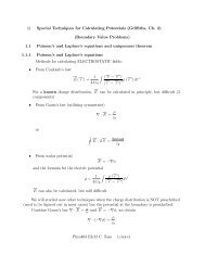
1Φ(z > 0)qq''ε0εrr32q'Φ(z < 0)Figure 5-3: Images q 0 and q 00 for a ‡at dielectric boundary.Solving Eqs. (5.7) and (5.13) for q 0 and q 00 , we …ndq 0 = 0 + 0(5.14)q 00 =2 + 0q (5.15)5.3 Image for Cylindrical Surfaces (Two Dimensional)The potential due to a long line charge (C/m) placed parallel to a grounded conducting cylindercan be found by the method of image. In Chapter 2, we saw that two opposite line charges of equalmagnitudes, + and create a family of equipotential cylindrical surfaces,(r + ; r ) = rln2 0 r +(5.16)where r + and r are the distances to the respective line charges, + and . Consider a linecharge at a distance 0 from the axis of a cylinder having a radius a. A negative line chargeat a distance 00 = a 2 = 1 and the positive line charge make the cylinder surface an equipotentialsurface s = aln2 0 0(5.17)(Check this by considering the potentials at A and B in Figure 5.4.) In order to make the cylindersurface at zero potential, we have to subtract this potential from the potential given in Eq. (5.16)which is based on the choice = 0 on the midplane, r + = r . Therefore, the solution to the4

potential becomesBut(r) = rln2 0 r +r = aln 1r + = 2 + 02 2 0 cos 1=2" 2 + a2 0 2(5.18)(5.19)2 a2 0 cos # 1=2(5.20)Substituting these into Eq. (5.18), we …nally obtain2 2 02 1=23(; ) =aln 62 + a 2 2 0 cos 2 0 4 ( 2 + 02 2 0 cos ) 1=2 75(5.21)When = a, this indeed vanishes.The surface charge density induced on the cylinder surface is given by@ = 0@=a=2 2 1a 02 + a 2a2a 0 cos (C/m 2 ) (5.22)Therefore, the total charge (per unit length) on the cylinder surface isql =2 02 a 2 Z 20 02 + a 2d2a 0 cos (5.23)The integral reduces to2 02 a 2 (5.24)when 1 > a. Therefore, the charge per unit length of the cylinder is simply, as expected.5.4 Image for a SphereWe consider a charge q at a distance r 0 from the center of a grounded conducting sphere of radiusa. The potential is symmetric about the line connecting the center and the charge. Therefore, animage charge should be on the same line. We assume a negative charge q 0 placed at a distance xfrom the center. The potential at the point A is A = 1 4 0r 0qa aq 0(5.25)x5

ρr ­r+ρ''−λρ'λaFigure 5-4: A line charge at a distance 0 from the center of a conducting cylinder of radius aand its image line charge at 00 = a 2 = 0 make the cylinder surface an equipotential surface at s =2" 0ln (a= 0 ) :This should vanish if the image is to replace the sphere without a¤ecting the potential outside thesphere. Therefore,Similarly, the potential at B is given byqr 0 a = q0a x B = 1 q4 0 D + a(5.26)q 0 = 0 (5.27)a + xqr 0 + a =Solving Eqs. (5.26) and (5.28) for x and q 0 , we …ndq0a + x(5.28)q 0 = a r 0 q (5.29)Therefore, a chargex = a2r 0 (5.30)aq=r 0 placed at a distance a 2 =r 0 from the center can be used to replace thesphere as far as the potential and electric …eld outside the sphere are concerned. Outside the sphere,the potential is given by =q 1 a=r 0 4 0 r + r(5.31)6

­r+Ba­qr''Ar'qFigure 5-5: Image for a sphere. Charge q at distance r 0 from the center of a sphere of radius a andits image q at r 00 = a 2 =r 0 make the potential vanish on the sphere surface r = a:where r 1 and r 2 are the distances between the observing point and respective charges, and given,in terms of the coordinate (r; ) at the observing point, byr + = r 2 + r 02 2rr 0 cos 1=2" ar = r 2 2 2# 1=2+r 0 2 a2r 0 r cos (5.32)The surface charge density on the sphere surface can be evaluated from() = 0@@r= 14r=ar 02 a qa(a 2 + r 02 2ar 0 cos ) 3=2 (5.33)Therefore, the total charge residing on the outer surface of the sphere is given by the integral,q s ===Z ()2a 2 sin d0r 02 Z 1a a 2 1d ( = cos )a1 (a 2 + r 02 2ar 0 3=2)ar 0 q = q0This result is expected from the Gauss’ law because thesphere surface.q 0 is the only charge enclosed by theExample7

The LHS is equal to Z r r + r2 dV (5.37)A charge q is placed at a distance D from the center of an isolated (‡oating) conducting sphere ofa radius a. When the sphere carries no charges, what will the sphere potential be?We …rst make the sphere potential zero by placing a charge q 0 = aq=D at r 0 = a 2 =D as inthe preceding discussion. Since the sphere carries no net charge, if a charge +q 0 = +aq=D is placedat the center of the sphere, the sphere potential will be raised (when q > 0) to s ==1 aq=D4 0 a1 q4 0 D(5.34)Note that this is independent of the sphere radius a. When the sphere carries a net charge Q, thesphere potential becomes s = 1 q4 0 D + Q a5.5 Green’s Theorem and Green’s Function(5.35)The method of image charges has a more important application in potential boundary value problems.When a potential is prescribed on a closed surface, it uniquely determines the potential in thespace surrounding the surface and also in the space surrounded by the surface. The most generalformulation for the potential is given in terms of a scalar function called Green’s function, whichis closely related to the potential due to a charge and its image for a given surface shape.For arbitrary scalar functions and , the following identity immediately follows from Gauss’theorem,ZIr (r )dV =r dS (5.36)Therefore,Zr r + r 2 IdV =r dS (5.38)Exchanging and , we obtainZr r + r 2 IdV =r dS (5.39)Substracting Eq. (5.39) from Eq. (5.38), yieldsZr 2 r 2 IdV =(r r) dS (5.40)This is known as the Green’s theorem. Its usefulness in potential problems can be appreciated asfollows.8

In Eq. (5.40), we identify as the desired scalar potential (r), and as a solution to thefollowing singular Poisson’s equationr 2 G = r r 0 (5.41)Since the potential (r) satis…es Poisson’s equation,r 2 = 1 0 (5.42)andZ(r 0 )(r r 0 )dV 0 = (r) (5.43)Eq. (5.40) yields,(r) = 1 0ZG(r; r 0 )(r 0 )dV 0I( s r 0 G Gr 0 s ) dS 0 (5.44)swhere s (r 0 ) is the surface potential prescribed on S, and r 0 indicates derivative with respectto the surface coordinates r 0 . When there are no surfaces, and the potential is entirely due to aprescribed charge density distribution , the Green’s function isG(r; r 0 ) = 14jr1r 0 j(5.45)and the potential is given by the familiar form,(r) = 14 0Z(r 0 )jr r 0 j dV 0 (5.46)In the absence of charges ( = 0), the potential is determined by the surface potential s andits derivative, r s , which is of course related to the electric …eld on the surface.The Green’s function in Eq. (5.45) is essentially the potential due to a charge located at r 0 .However, in addition to this particular solution, any general solutions satisfyingr 2 G g = 0 (5.47)can be added to the Green’s function so that it vanishes on a given surface. In this case (G = 0 onS), the potential due to a prescribed surface potential distribution becomes,(r) =I s (r 0 ) @G@n 0 dS0 (5.48)where n 0 is the normal vector on the surface, which is directed away from the region in which wewish to evaluate the potential. (Fig. 5.6) This is known as the Dirichlet’s formulation for potentialboundary value problems.9

Solving a boundary value potential problem is now reduced to …nding a suitable Green’s functionfor a given surface shape, on which G = 0. This is where the method of image will be very useful.Green’s Function for a SphereConsider a spherical surface having radius a. We place a charge q at r 0 . An image chargeq 0 =aq=r 0 atr 00 = a2r 02 r0 (5.49)and the original charge q at r 0 make the surface potential vanish. Therefore, the Green’s functionfor a sphere is immediately written asG(r; r 0 ) = 1 14 jr r 0 ja=r 0 jr r 00 j(5.50)Noting,r r 0 = r 2 + r 02 2rr 0 cos 1=2"r r 00 a= r 2 2 2+r 0(5.51)2 a2r 0 r cos # 1=2(5.52)Fig. 5.6 Geometry for the Dirichlet boundary value problems,Fig. 5.7 Greeen’s function for a spherical boundary is essentially equivalent to the potential dueto a charge near a grounded conducting sphere of the same radius.we …ndG(r; r 0 ) = 14= 140a1rB0@(r 2 + r 02 2rr 0 cos ) 1=2 r 2 + a 2 2r 002 a2r 0 r cos B11@(r 2 + r 02 2rr 0 cos ) 1=2 r 2 r 02+ aa 2 2rr 0 cos 21 1=2CA1C 1=2AWhen we wish to evaluate the potential outside the sphere, the normal derivative is given by@G@n 0 == 14= 1 a4@G r@r 00 =a1r 2Ba r cos r cos aC@(r 2 + a 2 2ra cos ) 3=2 (r 2 + a 2 2ra cos ) 3=2 Ar 2 1a (r 2 + a 2 2ra cos ) 3=2 (r > a) (5.53)For interior problems, the negative of the above equation is to be employed. Recall that cos in10

Eq. (5.53) is given bycos = cos cos 0 + sin sin 0 cos( 0 ) (5.54)in terms of the angular locations of the vectors r = (r; ; ) and r 0 = (r 0 ; 0 ; 0 ). Substituting Eq.(5.53) into Eq. (5.48), we …nally obtain the desired exterior potential,(r) = a2 r24 a Z Z 2a sin 0 d 0 d 0 s ( 0 ; 0 )00 (r 2 + a 2 2ra cos ) 3=2 (5.55)Let us apply this formula to the problem of oppositely charged hemisphere which we solved inChapter 3. The surface potential s () is described by,8+V 0 < < >< 2 s () =(5.56)>: V2 < < and is independent of the azimuthal angle . On the axis, = 0, and the potential becomes(z) = a2 z24 a " Z =2a 2Z 0sin 0 d 0z 2 + a 2 2az cos 0 3=2#sin 0 d 0=2 z 2 + a 2 2az cos 0 3=2 a2z 2 = Vz p z 2 + a + sign z 2(5.57)wheresign z =(+1 for z > 01 for z < 0(5.58)Note that the potential (z) must be an odd function of z. When z > a, Eq. (5.57) may beexpanded as 3 a 2 7 a 4(z) = V+ (5.59)2 z 8 zTherefore, at an arbitrary location (r > a; ), the potential is given by, 3 a 2(r; ) = V P1 (cos )2 r7 a 4P3 (cos ) + 8 r(5.60)which agrees with the previous result in Eq. (3.175). The interior potential (r < a) can immediatelybe written down by inspection as 3 r(r; ) = V2 a P 1(cos )7 r 3P3 (cos ) + 8 aGreen’s Function for a Long Cylinder (Two Dimensional)(5.61)11

The image line charge and corresponding potential due to a long line charge placed parallelto a grounded conducting cylindrical surface has been worked out in the preceding section. Thepotential is given bywherer = (; ) r; r 0 =r 0 = ( 0 ; 0 ) ar 00 2= ; 0 a jrln2 0 0 jr(observing point)r 00 jr 0 j(location of the line charge)(location of the image)Then, the Green’s function for a cylinder can be identi…ed as(5.62)G(r; r 0 ) = 1 a jr r 00 2 ln j 0 jr r 0 j1=2 ln 2 + 02 2 0 cos( 0 ) 1=2+ 1 22 ln 02 1=2a 2 + a 2 2 0 cos( 0 )(5.63)For exterior ( > a), the relevant normal derivative is@G@n = @G @ 0 0 =a= 12 2aa 2 + a 2 2a cos( 0 )( > a) (5.64)For interior, the negative of Eq. (5.64) is to be used.It is left for an exercise to recover the potential due to a cylinder, its upper half being at +Vand lower half at V , worked out in Chapter 3.12