electrostatics i electric field and scalar potential - Department of ...

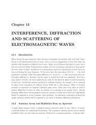
Chapter 1ELECTROSTATICS IELECTRIC FIELD AND SCALARPOTENTIAL1.1 IntroductionAtoms and molecules under normal circumstances contain equal number of protons and electrons tomaintain macroscopic charge neutrality. However, charge neutrality can be disturbed rather easilyas we often experience in daily life. "Static electricity" induced when walking on a carpet andcaressing a cat is a familiar phenomenon, and is known as frictional (or tribo) electricity. Beforethe invention of chemical batteries (Volta, 1786), electricity generation had been largely done byfrictional electricity generators. In nature, lightnings are caused by electrical discharges of electriccharges accumulated through friction among cloud particles. In frictional electricity, mechanicaldisturbance given to otherwise charge neutral molecules either splits electrons o¤ a material body,or adds them. For example, if an ebony rod is rubbed with a piece of fur, electrons are transferedfrom the fur to the ebony, and the ebony rod becomes negatively charged, while the fur becomespositively charged.Charge neutrality can be disturbed by various other means, such as thermal, chemical, opticaland electromagnetic disturbances. It is well known that even a candle ‡ame is weakly ionized(cuased by thermal ionization) and responds to an electric …eld. Chemical batteries are capable,through chemical reactions, of separating charges. Some metals are known to emit electrons whenexposed to ultraviolet light (photoelectric e¤ect discovered by Hertz in 1897 and later given quantummechanical explanation by Einstein). Finally, as an example of electromagnetic means of chargeseparation, the plasma (ionized gas) state in ‡uorescent lamps and plasma TV may be added tothe list.Charged bodies exert electric forces (Coulomb force) on each other. Systematic experimentson electric forces had been carried out by Cavendish and Coulomb in the 18th century and led1

to the establishment of the Coulomb’s law. Like charges repel each other, while unlike chargesattract each other. Therefore, in any attempt to separate charges out of an initially charge neutralbody, energy must be added. For example, in frictional electricity, mechanical energy is expendedto separate charges. In chemical batteries, chemical energy is converted into electric energy, andin electric generators, either gravitational (as in hydropower generation) or thermal (as in steampower plants) energy is converted into electric energy.The Coulomb force to act between two charges is inversely proportional to r 2 where r is theseparation distance between the charges. A hydrogen atom consists of one electron ”revolving”around a proton. The centripetal Coulomb force (attracting) is counterbalanced by the mechanicalcentrifugal force, and the electron stays on a circular orbit. (This is a classical electrodynamicmodel. For a more satisfactory description of a hydrogen atom, quantum mechanical analysis isrequired. However, the concept of force balance is basically correct.) A nucleus of heavier atomscontains more than one proton. The size of a nucleus is of order 10 15 m (compare this with theatomic size 10 10 m). Therefore, among the protons packed in a nucleus, a tremendously largerepelling Coulomb force should act, and some other force, which is not of electric nature, mustkeep protons together. This is provided by the so-called ”strong” nuclear force which acts amonghadrons such as protons and neutrons. Obviously, the nature of nuclear force is beyond the realm ofclassical electrodynamics. However, it should be realized that nuclear energy that can be releasedwhen a heavy nucleus (such as U 235 ) splits (nuclear …ssion process) is nothing but electric energystored in a nucleus.Electrostatics is one branch of electrodynamics in which electric charges are either stationaryor moving su¢ ciently slowly so that magnetic …eld induction and electromagnetic radiation can beignored entirely. All basic laws in electrostatics (Gauss’law, Maxwell’s equations) follow from theCoulomb’s law. Therefore, formulating the electric …eld and scalar potential in electrostatics will bededuced from this fundamental law. It should be pointed out that electrostatics (together with magnetostatics)provides us with preparation for more general electrodynamics, electromagnetic wavephenomena in particular. For example, electromagnetic wave propagation in a medium (includingvacuum) requires that the medium be able to store both electric and magnetic energy. Obviously,electric energy storage leads us to the concept of capacitance. Calculation of the capacitance of agiven electrode system is one important application of electrostatics, but the concept of capacitance(and inductance) will also play fundamental roles in dynamic electromagnetic phenomena.1.2 Coulomb’s LawIn the late 1700’s, Cavendish and, independently, Coulomb carried out extensive research on staticelectricity. (At that time, no batteries were available, and electricity generation was mainly donewith frictional electricity machines.) Apparently, Cavendish’s discovery of the inverse square law,now known as Coulomb’s law, was made before Coulomb. However, Cavendish did not publishhis large amount of work on electricity, while Coulomb wrote several papers on electricity andmagnetism. Of course, Cavendish is best known for his gravitational torsion balance experiments2

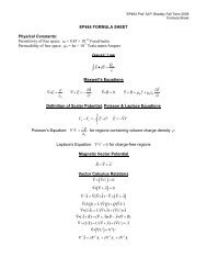
which experimentally veri…ed the inverse square law of gravitational force originally postulated byNewton. Both Cavendish and Coulomb used similar torsion balance apparatus to measure electricforces acting between charged bodies.Coulomb’s law is stated as follows. When two charges q 1 and q 2 are at a distance r from eachother, the electric force exerted on each other is proportional to q 1q 2r 2 ,F = const. q 1q 2r 2 : (1.1)In the MKS-Ampere unit system (SI unit system), the charge is measured in Coulombs (C), thedistance in meters (m), and the force in Newtons (N). In these units, the constant experimentallydetermined is N mconstant = 8:99 10 9 2C 2Figure 1-1: Repelling Coulomb force between like charges.The force is a vector quantity. In the case of the Coulomb force, the force is directed along theseparation distance vector r, and a more formal expression is given byF = const. q 1q 2r 2 e r (1.2)wheree r = r r(1.3)is the unit vector along the position vector r. Of course, both charges q 1 and q 2 experience aforce of the same magnitude, but oppositely directed. The sign of the product q 1 q 2 can be eitherpositive or negative. When q 1 q 2 > 0, the force is repelling, and when q 1 q 2 < 0, the force isattractive. In the 18th century when Cavendish and Coulomb conducted experiments, the presence3

of two kinds of charges, positive and negative, was known although their origin, namely chargedelementary particles, was clari…ed much later. The electron was discovered by Thomson in 1897.The electronic charge presently established is1:6 10 19 Coulomb.The proportional constant in the Coulomb’s law corresponds to the force to act between twoequal charges, 1 C each, separated by a distance of 1 m.By arranging such an experimentalsituation, the constant could be measured as done by Cavendish and Coulomb. (In more modernmethods, the velocity of light in vacuum provides an indirect measurement of the constant. Thiswill become clear later in Chapter 7.) In the MKS-Ampere unit system, the connection betweenmechanical force (Newtons) and basic electromagnetic unit is actually made in terms of magneticforce, rather than the Coulomb force, as will be explained in Chapter 7. When two long parallelcurrents of equal magnitude separated 1 m exert a force per unit length of 2 10 7 N/m, themagnitude of the current is de…ned to be 1 Ampere. The electric charge, 1 C, is then deducedfrom,1 C = 1 Ampere 1 secIn other unit systems, the Coulomb’s law itself is employed to de…ne the unit of electric charges. Forexample, in the CGS-ESU (ESU for ElectroStatic Unit) system, when two equal charges separatedby 1 cm exert a force of 1 dyne on each other, the charge is de…ned to be 1 ESU. Since 1 N = 10 7dyne, and 1 m = 10 2 cm, we can readily see that1 C =For example, the electronic charge in ESU is1 ESUp8:99 10 18 '1 ESU3:0 10 91:6 10 19 3:0 10 9 = 4:8 10 10 ESUAlthough in engineering, the MKS-Ampere (SI) unit system is universally accepted, the CGS-ESUand associated Gaussian unit system is still popular in physics. Both have merits and demerits,and it is di¢ cult to judge one unit system superior to the other.In the MKS-Ampere unit system, the Coulomb’s lawis rewritten aswhereF = 8:98 10 9 q 1q 2r 2 e r (N) (1.4)F = 14 0q 1 q 2r 2 e r (N) (1.5) 0 = 8:85 10 12 C 2N m 2 (1.6)is called the vacuum permittivity. The appearance of the numerical factor 4 may be uncomfortable,but cannot be entirely avoided. If we do not introduce the factor 4 in the Coulomb’s law, it willpop up in the corresponding Maxwell’s equation. In fact, the Maxwell’s equation for the static4

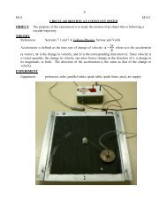
Figure 1-2: In MKS unit system, I = 1 Ampere current is de…ned if the force per unit length betweenin…nite parallel currents 1 m apart is 2 10 7 N/m. The magnetic permeability 0 = 4 10 7H/m is an assigned constant to de…ne 1 Ampere current.electric …eld in the CGS-ESU system has to be written asrE = 4 (1.7)because the factor 4 is avoided in the corresponding Coulomb’s law,F = q 1q 2r 2 e r (dynes)The newly introduced constant 0 is one of the fundamental constants in electrodynamics. Notethat 0 is a measured constant, since it is derived from the original measured constant, 8:99 10 9Nm 2 /C in the Coulomb’s law. The permittivity of air (room temperature, 1 atmospheric pressure)is about 1:0004 0 due to the polarizability of air molecules. For practical applications, the airpermittivity can be very well approximated by the vacuum permittivity.1.3 Electric Field EInterpretation of Coulomb’s law was a matter of debate before the concept of electric …eld waswell established by Faraday and Maxwell. Before Faraday and Maxwell, the so-called “theory ofaction at distance” once prevailed. According to this theory, electric e¤ects (such as Coulombforce) appear through some sort of direct interaction between charges, and space (or vacuum)has nothing to do with the interaction. In the “…eld” theory, a single charge “disturbs” spacesurrounding it by creating an electric …eld. The Coulomb force to act between two charges is due5

to interaction between one charge and the electric …eld produced by the other. The …eld theoryis now well accepted, and modern electrodynamics is almost entirely described by …eld quantitiessuch as electric and magnetic …elds.Let us write down the Coulomb force again,This can be written eitherorF = 1 q 1 q 24 0 r 2e rF = 14 0q 1r 2 e r q 2 (1.8)F = 14 0q 2r 2 e r q 1 (1.9)We may interpret Eq. (1.8) as the force experienced by a charge q 2 placed in an electric …eld,E 1 = 14 0q 1r 2 e r (1.10)produced by a charge q 1 while Eq. (1.9) as the force experienced by a charge q 1 placed in an electric…eld,produced by a charge q 2 .electric …eld given byregardless of the presence of a second charge.E 2 = 14 0q 2r 2 e r (1.11)A single charge q in the space with a permittivity thus produces anE = 14 0qr 2 e r (N/C) (1.12)Numerically, the electric …eld is equivalent to aforce to act on a unit change. Since the force is a vector, so is the electric …eld, and completedetermination of an electric …eld requires three spatial components.byIn general, if a charge q is placed in an electric …eld E, the force to act on the charge is givenF = qE (N) (1.13)This may alternatively be used for de…nition of an electric …eld, namely, if a stationary charge qexperiences a force proportional to the amount of the charge, then we de…ne that an electric …eld ispresent. (Elementary particles such as protons and electrons do have masses, and they experiencegravitational forces as well. However, gravitational forces are orders of magnitude smaller thanelectromagnetic forces, and in most practical applications, gravitational forces can be ignored.)Although Eq. (1.12) has been deduced from Coulomb’s law, the inverse is not always true, that is,electric …elds are not necessarily due directly to charges. A time varying magnetic …eld producesan electric …eld (Faraday’s law). Also, an object travelling across a magnetic …eld experiences anelectric …eld (motional electromotive force), as we will study in Chapter 9. However, regardless ofthe origin of the electric …eld, the force equation, Eq. (1.12), holds.6

E2E tq1PE1qFigure 1-3: Vectorial superposition of electric …eld.21.4 Principle of Superposition and Electric Field due to a DistributedChargeThe expression for the electric …eld due to a point charge,E = 14 0qr 2 e r (1.14)can be applied repeatedly to …nd an electric …eld due to a system of charges. For example, if thereare two charges q 1 at r 1 and q 2 at r 2 , the total …eld can be found from,Note that the quantities,E = 14 0r r 1jr r 1 j 3 q 1 + 14 0r r 2jr r 2 j 3 q 2 (1.15)r r 1jr r 1 j ; r r 2jr r 2 jare the unit vectors in the directions r r 1 and r r 2 , respectively. For larger number of charges,the total electric …eld can still be found as vector sum of electric …elds due to individual charges.This is known as the principle of superposition. For N discrete charges, the electric …eld can bewritten down as,E = 14 0N Xi=1r r ijr r i j 3 q i (1.16)As the number of charges increases, the summation becomes rather awkward. In most practicalapplications, the charge distribution can be regarded continuous, rather than discrete.As one7

would expect, the summation in the case of discrete charges can be replaced by an integral in thecase of a continuous charge distribution.,A continuous charge distribution can be described by a local charge density,(r) (C/m 3 )which may vary as a function of position r. Since the size of elementary particles is so small, acollection of those particles (e.g. electrons) can be well approximated by a continuous function(r), just as we treat water as a ‡uid although, microscopically, water consists of discrete watermolecules.Let us pick up a small volume dV 0 located at a distance r 0 from a reference point O as shownin Fig. 1.4. The charge contained in the volume dV 0 located at r 0 isdq = (r 0 )dV 0By choosing the volume element su¢ ciently small, we may regard the charge dq a point charge.We already know how to express the electric …eld due to a point charge,dE ==1 dq(r r 0 )4 0 jr r 0 j 31 r r 04 0 jr r 0 j 3 (r0 )dV 0 (1.17)Therefore, the electric …eld at r can be calculated from the following integral,ZE(r) =dE = 14 0Zr r 0jr r 0 j 3 (r0 )dV 0 (1.18)This is a general formula for calculating an electric …eld due to an arbitrary distribution of charges.Remember that we have derived it from the Coulomb’s law.Although the formula we just derived is a complete solution for static electric …elds due to acharge distribution, it is seldom used in practical applications except for simple (or often trivial)cases. There are several reasons for this. First, Eq. (1.18) is a vector equation. In the cartesiancoordinates, for example, three components, E x ; E y and E z will have to be evaluated separately.That is, we have to carry out integrations three times for a complete vector solution. Second, inmany potential boundary value problems, the charge distribution, (r), is not known a priori. Forexample, in evaluation of a capacitance of a given electrode system, the problem is reversed, thatis, we calculate the electric …eld (from the scalar potential) …rst, and then evaluate the chargedistribution on the surface of electrodes.As we will study in Section 2, the method based onthe scalar potential is more convenient in practical applications than evaluating the electric …eldusing Eq. (1.18). However, if the charge distribution is known, we can certainly use Eq. (1.18) toevaluate the electric …eld at an arbitrary point. Let us work on some simple examples.8

dEr ­ r'dq =ρdV'rr'OFigure 1-4: Di¤erential charge dq = dV 0 produces a di¤erential electric …eld dE:Charge SheetLet a large, thin insulating sheet carry a uniform surface charge density (C/m 2 ) (= constant).If the sheet is large enough, or the point at which we wish to evaluate the electric …eld is closeenough to the sheet, the electric …eld should be perpendicular to the sheet because of cancellationby an element located opposite with respect to the origin O. Choosing the cartesian coordinatesx; y; z, we then have to evaluate only the z component of the electric …eld at a distance z from thesheet.Let us pick up a surface element dx 0 dy 0 located at (x 0 ; y 0 ; z 0 = 0) on the sheet. The elementcarries a “point charge”dq = dx 0 dy 0 . Then, the magnitude of the electric …eld on the z axis is,and its z component is,dE = 14 0dx 0 dy 0x 02 + y 02 + z 2 (1.19)dE z = 1 z4 0 (x 02 + y 02 + z 2 ) 3=2 dx0 dy 0 (1.20)Therefore, the electric …eld on the axis is given by the following integral,E z =z Z 1 1dx4 0 1Z 0 dy 01 (x 02 + y 02 + z 2 ) 3=2 (1.21)However, the double surface integral can be replaced by a single integral over the radius r 0 , wherer 02 = x 02 + y 02 so thatE z =z Z 12r 04 0 0 (r 02 + z 2 ) 3=2 dr0 (1.22)9

The integral is elementary, and we …ndE z = z2 0= 2 0zjzj1 r 0 =1pr 02 + z 2r 0 =0(1.23)where p z 2 = jzj has been substituted.The solution indicates that the magnitude of the electric …eld is independent of the distancefrom the sheet. The direction of the electric …eld is negative in the region z < 0, and positive forz > 0. When there are two oppositely charged sheets, and (C/m 2 ), the electric …eld outsidethe sheets if zero, but the …eld in between the sheets is given by,E z = (1.24) 0as can be readily seen from the principle of superposition. This con…guration corresponds to aparallel plate capacitor provided the edge e¤ects are ignored.Line ChargeWe assume a long line charge with a line charge density (C/m). At a distance r from the linecharge, the di¤erential electric …eld due to a charge dq = dz located at z isdE = 1 dz4 0 r 2 + z 2 (cos e r + sin e z ) (1.25)where,cos =rpr 2 + z ; sin = zp 2 r 2 + z 2The z component is an odd function of z. Therefore, the z component of the electric …eld vanishesafter integration from z =1 to +1. The radial (r) component remains …nite, and is given by,E r = Z 1r4 0 1 (r 2 + z 2 dz =) 3=2 2 0 r(1.26)Remember that this result is valid only if the line charge is long, or the point of observation issu¢ ciently close to a line charge of …nite length.1.5 Gauss’Law for Static Electric FieldThe electric …eld at a distance r from a point charge q is,E = 14 0qr 2 e r;10

chargesheet σ(C/m 2 )E =σ/2ε 0E =σ/2ε 0σ−σE = 0E = 0E =σ/ε 0Figure 1-5: Upper …gure: Single charge sheet. The electric …eld on both sides is E z = =2" 0 : Lower…gure: Equal, opposite charge sheets. The …eld in-between is E z = =" 0: Outside, E z = 0:dE rdEdEzdq=λdzzrline chargezFigure 1-6: Electric …eld due to a long line charge (line charge density C/m). Note that E z = 0and the radial electric …eld E r = can also be found using Gauss’law.2" 0 r11

dE nrθγaqbFigure 1-7: Gauss’law applied to a sphere that is not concentric with the charge. Note r cos +b cos = a:On a spherical surface with radius r, the magnitude of the electric …eld is constant, and the quantity,4r 2 E ris equal to q= 0 . This strongly suggests that the closed surface integral of the electric …eld,IEdS (1.27)is equal to the amount of charge enclosed by the closed surface S divided by 0 ,IEdS = qS " 0SNotingandISZEdS =Zq =r EdV (r) dVwe …nd the Maxwell’s equationr E = " 0Let us see if this is the case for a spherical surface which is not concentric with the point chargeq. We denote the distance between the charge and the spherical center by b, and the radius of thesphere by a.The electric …eld on the surface is no more uniform. It is not normal to the surface, either. Noting12

the relationship,r 2 = a 2 + b 22ab cos in Fig. ??, we …nd the magnitude of the electric …eld at angle ,E =q 14 0 a 2 + b 2 2ab cos (1.28)The component normal to the spherical surface is E cos where the angle is related to throughTherefore, the entire surface integral reduces to,ISE dS =q Z 4 0r cos + b cos = a:0a b cos (a 2 + b 2 2ab cos ) 3=2 2a2 sin d (1.29)wheredS = 2a 2 sin dis the area of the ring having radius asin and width ad. The relevant integral isZ 0(a b cos ) sin (a 2 + b 2 2ab cos ) 3=2 d = 8 b0; a < b(1.30)(In integration, it is convenient to change the variable from to through = cos . Then theintegral reduces to=1b p a 2 + b 2R 11a b(a 2 + b 2 d2ab) 3=2 11 a 2 + b 22aba 2 pb a 2 + b 21ab2ab11Evaluation of the de…nite integral is left for a mathematical exercise. Note that p (a b) 2 = ja bj.)Therefore, the surface integral of the electric …eld becomes,I8< q; a > bEdS = 0: 0; a < b(1.31)Obviously, the case a > b corresponds to a sphere enclosing the charge, and a < b corresponds tothe case in which the charge is outside the closed spherical surface. The result may be generalizedto a closed surface of an arbitrary shape. The following formula is called Gauss’law, 0ISEdS = qTotal chargeenclosed by S!(1.32)13

Again, remember that Gauss’ law is equivalent to Coulomb’s law, since we have “deduced” theformer from the latter. In fact, Gauss’law can be mathematically “proven”if we adopt Coulomb’slaw. A formal proof will be given after the Maxwell’s equation is introduced.Gauss’law can be convenient for simple cases in which a system has a high degree of symmetry,such as spherical, cylindrical, and planar symmetries. Let us work on a few simple examples.Uniformly-Charged Insulating SphereLet an insulating sphere of radius a carry a uniform charge density (C/m 3 ) and a total chargeq = 4 3 a3 (C). The system has complete spherical symmetry, and the only nonvanishing componentof the electric …eld is the radial component, E r . Outside the sphere (r > a), Gauss’law yields,4r 2 E r = q 0orE r =q4 0=a33 0 r 2 (1.33)which is identical to the …eld due to a point charge q concentrated at the center. Inside the sphere(r < a), Gauss’law reads4r 2 E r = 1 043 r3 (1.34)since in the RHS, only the amount of charge enclosed by the spherical surface (called Gaussiansurface) having a radius r (< a) enters. Solving for E r , we obtain,E r =3 0r (1.35)Therefore, in the sphere, the …eld linearly increases with the radius r up to the surface, r = a, wherethe interior …eld connects to the exterior …eld without dicontinuity. The electric …eld is maximumat the surface as shown in Fig. 1-8.The fact that the electric …eld should vanish at the center of a charged (uniformly!) sphere isunderstandable from spherical symmetry. At the center, the contribution from a charge dq to theelectric …eld can always be cancelled by another located opposite with respect to the center. Byanalogy, the gravitational …eld due to the earth mass itself at the earth’s center should be zero.Charged Conducting SphereA charge given to a conductor must reside entirely on the conductor surface so that the electric…eld inside a conductor body should be identically zero in static condition. If an electric …eld werenot zero in a conductor, a large electric current would ‡ow according to Ohm’s law,J = E (1.36)where (Siemens/m) is the conductivity. of metals is large. (For example, copper has '5:9 10 7 S/m). Therefore, unless E = 0 in a conductor, a large current should ‡ow, and thisviolates the assumption of static electricity. In other words, an electric …eld can exist in a conductor14

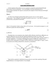
ErE maxa 2a 3a 4arρaFigure 1-8: Electric …eld of a unifrmly charged sphere. The …eld is 0 at the center. The maximum…eld, E max = a3" 0; occurs at the surface.only in dynamic conditions in which current ‡ow is allowed.If an excess charge q is given to a conducting sphere, the charge uniformly resides on the surfaceas a surface charge, with a surface charge density s = q=4a 2 (C/m 2 ) where a is the sphere radius.The electric …eld inside (r < a) the sphere is zero, while outside (r > a), it is given byE r = 14 0qr 2 (r > a) (1.37)Note that there is a sudden jump in the …eld at the surface (r = a) where the surface charge densityexists. In general, wherever an in…nitesimaly thin surface charge layer exists, the electric …eld therebecomes discontinuous. We will come back to this subject in Chapter 3 where the concept of thedisplacement vector D is introduced.Experimental Veri…cation of Coulomb’s Inverse Square LawAs stated earlier, Gauss’law and Coulomb’s law are physically identical, in the sense that theformer is derivable from the latter. Therefore, if Gauss’law can be veri…ed experimentally, thenCoulomb’s law is indirectly veri…ed also. Here, we are particularly concerned with a question: Howvalid is the inverse square law? Or put alternatively, when the Coulomb’s law is written asF = const:r n e rhow close is the power n to 2.0? Is it exactly 2.0? Experiments in the past have shown that n is15

ErE maxa 2a 3a 4arσaconducting spherecarrying a surfacechargeFigure 1-9: Electric …eld in a charged conducting sphere is 0. The charge q given to the spheremust reside on the surface as a surface charge = q=4a 2 C/m 2 :indeed very close to 2.0 with an uncertainty of order 10 16 . The power n is probably exactly equalto 2.The experiment performed by Plimpton and Lawton in 1936 was to measure the intensity ofelectric …eld inside a charged conducting shell. As we have just seen in the preceding example, anexcess charge given to a conductor must reside entirely on its outer surface, and the electric …eld inthe conductor must be zero. This holds for a conducting shell, too, and no charge can exist on theinner surface of the shell. Plimpton and Lawton established n = 2210 9 . Further improvementn = 2 2 10 16 was achieved later in 1971 by Williams et al.1.6 Di¤erential Equations for Static Electric Fields-Maxwell’s EquationsFor a given charge distribution (r), the electric …eld can be uniquely evaluated fromE(r) = 14 0Z r r0jr r 0 j 3 (r0 )dV 0 (1.38)as we have seen in Sec. 1.4. The electric …eld also satis…es Gauss’law,ISEdS = 1 0ZV(r)dV (1.39)16

We may use either formulation in evaluating the electric …eld due to a prescribed charge distribution.The electric …eld is a vector quantity. A vector can be uniquely de…ned if its divergence andcurl are both speci…ed. This mathematical theorem is known as Kirchho¤’s theorem. (Kirchho¤is a familiar name in electric circuit theory. However, his contributions are not limited to circuittheory, but quite diversi…ed.Kirchho¤’s scalar di¤raction formula for electromagnetic waves isanother important contribution, and had been used extensively until it was replaced by a moreaccurate vector di¤raction formula rather recently. See Chapter 13.) A derivation of vector di¤erentialequations for electric and magnetic …elds was formulated by Maxwell in the celebrated book“Treatise on Electricity and Magnetism” published in 1873.Each …eld (electric and magnetic)requires both divergence and curl. Therefore, for complete description of electric and magnetic…elds, four Maxwell’s equations emerge.In electrostatics, the magnetic …eld is absent (or ignored). Let us start with the divergence ofstatic electric …elds. In the example of a charged sphere in Sec. 2.5, we have seen that the electric…eld inside a uniformly charged spherical body can be found from Gauss’law,with the result,4r 2 E r = 1 043 r3 (1.40)E r =3 0r (1.41)Eq. (1.40) holds no matter how small r is chosen. The divergence of the electric …eld is de…ned bydiv E = r E =limV !0HS E dSV(1.42)In Eq. (1.40), the LHS is a special case of symmetric surface integration, and the quantity 4r 3 =3in the RHS is of course the volume. Therefore, if we take the limit of r ! 0 in the ratio,4r 2 E rlimr!0 43 r3it reduces to the de…nition of divergence. Consequently, the divergence of the electric …eld satis…es,r E = 0(1.43)This is one of Maxwell’s four equations.,Outside the charged sphere, the surface integration,IE dSSvanishes unless S intersects the sphere. Therefore, outside the sphere, r E = 0, as requiredbecause = 0 outside the sphere.The divergence equation alternatively follows from Gauss’ law, although physical meaning is17

less clear. The surface integral can be rewritten in terms of a volume integral as follows,I ZEdS =SVr E dV (Gauss’theorem) (1.44)This is a mathematical theorem, and has nothing to do with the physical Gauss’law, although theyare intimately related. Using this transformation, we can rewrite Gauss’law as,Zr E dV = 1 Z dV (1.45) 0Therefore, r E = = 0 immediately follows.The third method to derive the divergence equation for the electric …eld is to directly take thedivergence of Eq. (1.18),r r E(r) = 1 Zr r 4 0r r 0jr r 0 j 3 (r0 )dV 0 (1.46)where the subscript r indicates di¤erentiation with respect to the observer’s coordinates r. Thefunction, r r0r r jr r 0 j 3(1.47)has a peculiar property. It vanishes wherever r 6= r 0 but is not properly de…ned where r = r 0 . (Infact, it diverges at r = r 0 .) Introducing jrr 0 j = R, we indeed see that, r r0r r jr r 0 j 3 = 1 dR 2 1 R 2 dR R 2 = 0 (R 6= 0)However, its volume integral is well de…ned and remains …nite since R r r0rr jr r 0 j 3 dVI r r0=jr r 0 j 3 dSI I1=R 2 R2 d = d = 4 (1.48)where d is the di¤erential solid angle, and 4 is the total solid angle. In other words, the function,has the property of the delta function, r r0r r jr r 0 j 3(1.49) r r0r r jr r 0 j 3 = 4(r r 0 ) (1.50)18

where(r r 0 ) = (x x 0 )(y y 0 )(z z 0 ) (1.51)is the three-dimensional delta function having the dimensions of m 3 . Therefore, the integral inEq. (1.46) can be readily performed asZ44 0(r 0 )(r r 0 )dV 0 = 1 0(r) (1.52)and Eq. (1.46) is equivalent tor E = 1 0 (1.53)We now evaluate the curl of a static electric …eld given in Eq. (1.18). Taking the curl of bothsides, we …nd,However, in the RHS, the vector, r r0r r jr r 0 j 3r r E(r) = 14 0Z= r rjr r r0r r jr r 0 j 3 (r 0 )dV 0 (1.54)1r 0 j 3 (r r 0 1) +jr r 0 j 3 r r (r r 0 ) (1.55)identically vanishes, because the vector,r rjr1r 0 j 3= 3 r r0jr r 0 j 4 (1.56)is parallel to the vector rr 0 , andr r (r r 0 ) 0 (1.57)identically. In contrast to the divergence in Eq. (1.46), r r0r r jr r 0 j 3 0 (1.58)holds even at rr 0 = 0. Therefore, for static electric …elds due to charge distributions, we conclude,r E = 0 (1.59)We thus have speci…ed both divergence and curl of static electric …elds in Eqs. (1.53) and (1.59),respectively, which determine static electric …elds (vector) uniquely. The divergence equation holdsfor any electric …elds (electrostatic and non-electrostatic), but the curl equation is the special caseof the more general Maxwell’s equation,r E =@B@t(1.60)In static phenomena, @=@t = 0, and r E = 0 holds only for static electric …elds.19

What are the physical meanings of the Maxwell’s equations? The nonvanishing divergence ofthe static electric …eld indicates that the charge density is the source (or sink) of the …eld. Thismay be illustrated by the electric lines of force. A positive charge “emits”electric …eld lines, whilea negative charge “absorbs”electric lines of force, just like stream lines in water ‡ow. If two equal,but opposite charges are near by, the …eld lines “emitted”by the positive charge are all “absorbed”by the negative charge. If the magnitude of the charges are not equal, some …eld lines are notabsorbed by the negative charge.The vanishing curl of static electric …elds indicates that an electric …eld line does not close onitself, that is, a …eld line does not form a loop. (This is in contrast to non-electrostatic …eld forwhich the curl is nonvanishing.) In other words, static electric …eld lines always have heads or tailsas clearly seen in the above examples. Static …eld lines start at a positive charge and end at anegative charge.1.7 Scalar Potential (r)The vanishing curl of static electric …elds has an important implication. Since the curl of a gradientof an arbitrary scalar function is identically zero,r rF 0 (1.61)a static electric …eld (vector!) can be deduced from a gradient of some scalar function. We denotethis scalar by (r) and call it a scalar potential. The electric …eld is given by the gradient of thescalar potential,E(r) = r(r) (1.62)The negative sign is introduced so that the electric …eld is directed from higher to lower potentialregions, just like in the familiar gravitational …eld and gravitational potential.The dimensions of the scalar potential areNewton meterCoulomb= JouleCoulombThis is rede…ned as Volts (after Volta). Therefore, an alternative unit for the electric …eld isVolts/meter.The physical meaning of the electric …eld is (as discussed before) the force to act on a unitcharge. Then, the scalar potential can be interpreted as the work required to move a unit chargefrom one point to another, since(r) = (r 1 )Z rr 1E dr (1.63)where (r 1 ) is the potential at r 1 . Clearly, the potential is a relative quantity and is referredto the potential at a speci…ed reference point. (Again, the analogy to the gravitational potential20

VEdΦ(x)V0 dxFigure 1-10: Potential (x) = V d x and electric …eld E x =V=d in a parallel plate capacitor.should be recalled. When we measure the height of a mountain, usually the sea level is chosen asthe reference point.)As an example, let us consider a point charge q placed at the origin r = 0. The electric …eld isgiven by,E r (r) = 14 0qr 2 ; V/mIf the reference potential = 0 is chosen on a surface with a radius r 1 , the potential at an arbitrarypoint r becomes(r) ==Z rq 1r 14 0 r 2 dr q 1 14 0 r r 1(1.64)For a charge system of a …nite spatial extent, it is convenient to choose = 0 at r 1 = 1, so thatrelative to the zero potential at r = 1.(r) = 1 q; (V) (1.65)4 0 rSimilarly, the potential due to a charged conducting sphere with a total charge q and radius ais given by,(r) = 14 0qr(1.66)21

elative to = 0 at r = 1. The sphere potential can be found by equating the radius to r = a, sphere = 14 0qa(1.67)Note that this result is independent of whether the conducting sphere is solid or shell, since theelectric …eld in the conductor must vanish identically. In general, the potentials at any points onand in a conductor must be equal because E = 0 in a conductor. In particular, the surface of aconductor, no matter how complicated is its shape, is an equipotential surface. This fact will playan important role in potential boundary problems in Chapter III.In the following, we will work on a few examples in which the potentials can be calculated fromknown electric …elds.Potential of a Charged Insulating SphereThe electric …eld for this problem has been worked out in Sec. 1.5, and given by8>: a 3; (r > a)3 0 r2 3 0r; (r < a)(1.68)where is the charge density and a is the sphere radius. We choose = 0 at r = 1. Then, theexterior potential becomesZ r a 3(r) =1 3 0 r 2 dr= a 3; (r > a) (1.69)3 0 rOn the surface of the sphere, the potential takes the value,(a) = 3 a2 (1.70)Therefore, the interior potential becomes,(r) = (a)= a23 0= a22 0Z rrdra 3 0r 2 a 26 0r 2 ; (r < a) (1.71)6 0The potential at the sphere center is ,(r = 0) = a22 0(1.72)which is the maximum (if q > 0) potential. Note that the integration should be carried out starting22

at the reference point (r = 1 in this case), and radially inward.Potential due to a Long Line ChargeThe electric …eld due to a long line charge has been found in Section 1.5, and given byE = 12 0 (1.73)where (C/m) is the line charge density. Let us choose a reference, zero potential surface at aradius = a. (a cannot be in…nity, in contrast to the case of spheres, because the potential due toan in…nitely long line charge does not vanish at in…nity, but diverges. Such a line charge requiresin…nitely large amount of energy, and thus is of mathematical interest only.) Then, the potentialat an arbitrary radial position can be found as() ===Z aE dZ a12 0 d aln2 0 (1.74)The zero potential surface can be chosen arbitrarily, since the potential is a relative quantity.However, the potential di¤erence between two radial positions is independent of the choice of thereference. Indeed, the potential di¤erence between two points at 1 and 2 becomes( 1 ) ( 2 ) =in which the particular radius a has disappeared.=2 0ln2 0 aln 12 1 aln 2(1.75)In practical applications, the potential we just found can be used to calculate the capacitanceof a coaxial cable. Let us consider a coaxial cable having inner and outer conductor radii a and b,respectively, as shown in Fig. 1-11. We connect a dc power supply of a voltage V between the twoconductors. If we can calculate the charges q to appear on respective conductors, the capacitancecan be calculated by de…nition from,The charge per unit length is,C = q V = q l(F) (1.76)(1.77)Therefore, the potential di¤erence between the two conductors becomes,V = (a) (b) = bln2 0 a23

lV2abFigure 1-11: Coaxial cable.orHence,V =or the capacitance per unit length is given by,q b2 0 l ln a(1.78)C = q V = 2 0l (F) (1.79)lnb aCl= 2 0 (F/m) (1.80)lnb aIf the space between the conductors is …lled with a dielectric having a permittivity , this shouldbe modi…ed asCl= 2lnb (1.81)a1.8 Potential due to a Prescribed Charge DistributionIn the preceding Section, we have (brie‡y) learned how to calculate the potential (r) from a knownelectric …eld. However, in most applications, it is more common to reverse the procedure, namely,we …rst …nd the potential , and then calculate the electric …eld from,E = r (1.82)There are several reasons for inverting the procedure. The basic Maxwell’s equations for staticelectric …elds are,rE = 0(1.83)rE = 0 (1.84)24

Obviously, these are vector di¤erential equations, and for a complete solution, we must solve threedi¤erential equations for each component of the …eld E. However, if we substituteE =rinto rE = 0, we …nd a single scalar di¤erential equation for ,r 2 = 0(1.85)This is known as Poisson’s equation, and mathematically speaking, it is an inhomogeneous versionof the Laplace equation,r 2 = 0 (1.86)for which exhaustive studies have been made since the 18th century. The Laplace and Poisson’sequations most frequently appear in physical science and engineering. Analytic solutions to thoseequations can be found in a relatively limited number of cases. However, with powerful computersbecoming more easily accessible these days, numerical solutions to Poisson and Laplace equationsare no more prohibitively expensive even for complicated geometries for which analytic solutions areextremely di¢ cult, if not impossible. We will return to the problem of solving Laplace equations inthe following Chapter. Here, we derive a formal solution to the Poisson’s equation, which enablesus to calculate the potential for a prescribed charge distribution.There are several methods to …nd the solution tor 2 = 0and we start with a method that is physically most transparent. We have already seen that thepotential due to a point charge q is given by(r r 0 ) = q 14 0 jr r 0 j(1.87)where r 0 is the location of the point charge.For a distributed charge, we pick up a small volume dV 0 in the region where the charge density,, exists. The charge contained in the volume dV 0 isdq = dV 0 (1.88)By choosing the volume dV 0 su¢ ciently small, the di¤erential charge dq approaches a point charge.Therefore, the potential due to the charge dq located at r 0 becomesd = 14 0(r 0 )jr r 0 j dV 0 (1.89)25

dΦr ­ r'dqrr'Oprovided the reference potential = 0 is at r = 1. By integrating Eq. (??) over the dummyvariable r 0 , we …nd(r) = 14 0Zwhich is the desired solution to the Poisson’s equation.(r 0 )jr r 0 j dV 0 (1.90)The same result can be deduced from the electric …eld due to a prescribed charge distributionfound earlier,SinceE(r) = 14 0Zr r 0jr r 0 j 3 (r0 )dV 0 :r r 0 1jr r 0 j 3 = r rjr r 0 jwhere the subscript r indicates di¤erentiation with respect to the observing point r, we …ndE(r) =Z1r r4 0(r 0 )jr r 0 j dV 0 (1.91)Note that the di¤erential operator r r can be taken out of the integral, because it operates on ronly. Comparing with the basic relationship,E =rwe readily obtain(r) = 14 0Z(r 0 )jr r 0 j dV 0which is identical to Eq. (1.90). Below, we will apply this formula to a few simple problems.Potential due to a Line Charge of Finite LengthConsider a line charge of length 2a carrying a uniform line charge density (C=m). A di¤erential26

dΦadqz'ρz­aFigure 1-12: Line charge ( C/m)of …nite length 2a: dq = dz 0 :charge dq = dz 0 located at z 0 creates a potential at the coordinates (; z),d = 14 0dz 0p 2 + (z z 0 ) 2 (1.92)Integrating this over z 0 from z 0 =(; z) ===a to +a, we …ndZ adz 0p4 0 a (z 0 z) 2 + 2h pln (z 0 z)4 2 + 2 + z 0 z0p ! (z a)ln2 + 2 + a zp4 0 (z + a) 2 + 2 a zi aa(1.93)Let us examine special cases of the potential. At a point very close to the line charge, so thatz ! 0, and a, the potential reduces toThe potential of the form() '() = 2aln2 0 ( a) (1.94)2 0ln + const. (1.95)has been worked out in Sec. 2.6 for a long coaxial cable, and the result we just obtained is thereforeof an expected form.Far away from the line charge so that ; z a, we expect to recover the potential due to a27

point charge, q = 2a. On the plane z = 0, the logarithmic function approachesp !ln2 + a 2 + ap 2 + a 2 a' ln 1 + 2a ' 2a ( a) (1.96)Therefore, the potential indeed approaches() 'q 14 0 ( a) (1.97)where q = 2a is the total charge carried by the line. On the z axis, ! 0, and at jzj a, thepotential also approaches,(z) =='4 0lim4 0lnq 14 0 z!0ln1 + 2azCapacitance of a Thin Linear Conductorp !(z a) 2 + 2 + a zp(z + a) 2 + 2 a z(1.98)The expression for the potential in the vicinity of a line charge, Eq. (1.94), can be directly usedto …nd the capacitance of a thin linear conductor having a radius b and length 2a with a b. Onthe surface of the conductor, = b. Therefore, the potential of the conductor can be approximatedbyand the approximate capacitance is given by( = b) = 2aln2 0 b q 2a'4 0 a ln b 2aC = 4 0 a= lnb= 2" 0Lln(L=b)(1.99)where L = 2a is the total length of the conductor.Capacitance of Parallel Wire Transmission LineAs an application of the potential due to a line charge, we consider a long, two-parallel-wiretransmission line, which is often encountered in high voltage power transmission and old-fashionedtelephone lines. The geometry is shown in Fig. ??. We assume two thin parallel conductor wires28

of an equal radius a separated a distance d. By “thin conductor wires”, we mean d a. Since thecapacitance we are concerned here is the mutual capacitance between the two wires, we let the twowires carry equal, but opposite line charge densities, + and (C/m). Then, the potential atarbitrary point can be written down as(r + ; r ) ==[ ln r + + ln r ]2 0 rln2 0 r +where r + and rare the distance from the observing point to the positive and negative wires,respectively. Note that the reference, zero potential surface is chosen at the midplane on whichr + = r .When the wire radius a is small compared with the separation distance d, the potential at thesurface of the positive wire can be found by letting r + = a and r = d, + = dln2 0 a(1.100)Similarly, the potential at the negative wire is, = a=2 0 d dln2 0 a(1.101)Therefore, the potential di¤erence between the wires isV = + = dln 0 a(1.102)and the capacitance per unit length of the transmission line is given by,Cl= dV = 0= lna(F/m) (1.103)The capacitance (per unit length) of a single wire transmission line placed above the groundat a height h can be found in a similar manner. The ground potential can be chosen to be zero.Therefore, the potential di¤erence between the wire and the ground is given byV = 2hln2 0 a(1.104)where 2h is the distance between the wire and an image line charge located at the mirror point,z =h, in the ground. Then, the capacitance becomesCl 2h= 2 0 = lna(1.105)29

+λ r r­+ −λdFigure 1-13: Parallel wire transmission line. Separation distance d and wire radius a:Note that this is twice as large compared with the capacitance of the two-wire transmission line.The latter can be considered to be a series connection of two capacitors, one between the positivewire and the midplane, and the other between the negative wire and the midplane. The midplane,which is chosen at zero potential, can be replaced by a grounded large conducting plate withouta¤ecting the potential and electric …eld. The method of images will be discussed more fully inChapter 5.Both formulae in Eqs. (1.103) and (1.105) are subject to the assumption of thin wire radius,a d; h. As the wire radius becomes large, they become inaccurate, but only logarithmically. Forexample, the exact capacitance of the parallel wire transmission line is given byCl1= 0 "d + p # (1.106)dln2 4a 22aEven when a = 0:2d (thick conductors indeed), the error caused by using the approximate formulain Eq. (1.103) is less than 3%.Electric DipolesTwo charges of opposite signs, but equal magnitude, +q and q separated by a small distancea constitute an electric dipole. (A single charge q is called a monopole. Higher order multipoles,quadrupole, octapoles, etc., can be similarly constructed.) Dipoles are the basic elements in dielectricmaterials as we will study in detail in Chapter 4.jsin jThe potential due to two charges, +q and(r + ; r ) =q, can be written down asq 1 14 0 r + r(1.107)30

Φr++q­qa θr−Figure 1-14: Electric dipole consists of two charges q and q separated by a small distance a:where r + and rrelated throughare the distances to the respective charges from the observation point. They arer 2 + = r 2 + a 2 2ar cos (1.108)where is the angle between the z axis and the vector r . So far, we have not made any approximations,and Eq. (??) is exact.At a point far away from the dipole such that r + ; r a, r + may be approximated byr + ' r a cos (1.109)Then, the potential at r a becomes(r; ) ='q 1 14 0 r a cos rq a cos 4 0 r 2 (1.110)where we have replaced r(' r + ) by r. In contrast to the monopole potential,(r) = 14 0qrthe dipole potential is proportional to 1=r 2 , and thus of higher order in the series expansion inpowers of 1=r. The potentials due to the equal but opposite charges cancel each other in the lowest(monopole) order. Also, the dipole potential has the angular dependence, cos . It is convenient tointroduce the dipole moment (vector)p = qa (1.111)31

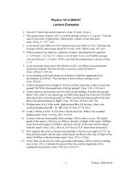
y1.00.80.60.40.2­0.6 ­0.4 ­0.2 0.2 0.4 0.6­0.2 x­0.4­0.6­0.8­1.0Figure 1-15: Equipotential surfaces of electric dipole p z :where a is the vector directed from the negative chargethe angle between a and r, we may rewrite Eq. (1.110) asq to the positive charge +q. Since is = 14 0p rr 3 (1.112)wherep r = pr cos = aqr cos The equipotential surface of the dipole is shown in Fig. 1.17.pjsin jThe electric …eld associated with the dipole can be calculated by taking the gradient of thepotential,E = r(r; )@= e r@r + e @ 1 aqr @ 4 0 r 2 cos = aq 24 0 r 3 cos e r + sin r 3 e (1.113)32

The electric …eld lines are described by the following di¤erential equation,dr= rd(1.114)E r E since the electric …eld is tangent to the …eld lines. The components, E r and E areE r =aq 2cos (1.115)4 0 r3 E =aq 14 0 r 3 sin Substituting these into Eq. (??), we …nd the following di¤erential equation to describe the …eldline,dr = 2r cot dorIntegrating both sides, we obtainordrr= 2 cot d (1.116)ln r = ln(c sin 2 ) (1.117)r = c sin 2 where c is a constant. The electric …eld lines of the diople are shown in Fig. 1.18. Note that theelectric …eld lines are normal to the equi potential surfaces.cos 2 1.9 Linear QuadrupoleCharges +q; 2q; and +q placed along the z axis at z = a; 0; a constitute a linear quadrupole.The potential at r a can be found as superposition of 3 potemtials, (r; ) ='q1p4" 0 r 2 + a 2 2ar cos qa2 3 cos 2 14" 0 r 3where use is made of binomial expansion2r + 1pr 2 + a 2 + 2ar cos 1p 1 + x= 112 x + 3 8 x2 33

y0.30.20.1­1.0 ­0.8 ­0.6 ­0.4 ­0.2 0.2 0.4 0.6 0.8 1.0­0.1­0.2­0.3xFigure 1-16: Electrif …eld lines of the diople p z = qa:Note that the dipole potemtial vanishes. This is because the quadrupole consists of two dipolesoppositely directed. The equipotebtial surfaces of the linear quadrupole is shown in Fig. 1.1 3 sin 2 y21­1.0 ­0.5 0.5 1.0x­1­2The functionP 2 (x) = 1 2 3x21 is the Legendre polymonial of order l = 2: The binomial expansion of the potential due to the34

charge q at z = a is 1 ===q1p4" 0 r 2 + a 2 2ar cos q 14" 0 r + a a2 3 cos 2 cos +r2 r 3 + 2q X1 a l4" 0 r l+1 P l (cos )l=0Likewise 2 ==q1p4" 0 r 2 + a 2 + 2ar cos q X1 ( 1) l a l4" 0 r l+1 P l (cos )l=035