- Page 2 and 3:
BASICS OFMATLAB®and Beyondc○ 200
- Page 4 and 5:
Library of Congress Cataloging-in-P
- Page 6 and 7:
typing pwd (print working directory
- Page 8 and 9:
ContentsIBasics of MATLAB1 First St
- Page 10 and 11:
20 Time-Frequency Analysis21 Line A
- Page 12 and 13:
39Answers to Exercises (Part I)40 A
- Page 14 and 15:
Set → Getting Started with MATLAB
- Page 16 and 17:
1.5 The Colon OperatorTo generate a
- Page 18 and 19:
matlab will recall the last command
- Page 20 and 21:
a = zeros(2,3)a =0 0 00 0 0>> b = o
- Page 22 and 23:
[a a(a)]ans =1 2 3 1 4 74 5 6 2 5 8
- Page 24 and 25:
a + bans =11 3344 6677 993.8 Transp
- Page 26 and 27:
4.2 Adding PlotsWhen you issue a pl
- Page 28 and 29:
x = [[1 2 3 4]’ [2 3 4 5]’ [3 4
- Page 30 and 31:
4.7 AxesSo far we have allowed matl
- Page 32 and 33: v =1122>> v*uans =1 2 0 11 2 0 12 4
- Page 34 and 35: max returns a vector containing the
- Page 36 and 37: s = 100*spiral(3)s =700 800 900600
- Page 38 and 39: We can plot the surface z as a func
- Page 40 and 41: The contour function plots the cont
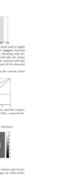
- Page 42 and 43: m = gray(8);colormap(m)imagesc(1:10
- Page 44 and 45: hold onplot3(x(ind),y(ind),z(ind),
- Page 46 and 47: z = 5*ones(3,3)z =5 5 55 5 55 5 5>>
- Page 48 and 49: contour(x,y,z,30);You may have noti
- Page 50 and 51: variables that are local to themsel
- Page 52 and 53: SwitchThe basic form of a switch st
- Page 54 and 55: i =i =123136Vectorised Codematlab i
- Page 56 and 57: 9.1 MATLAB FormatTo save all the va
- Page 58 and 59: 11 StartupEach time you start matla
- Page 60 and 61: Where p i is the population for yea
- Page 62 and 63: NaNs by leaving them off the plot.
- Page 64 and 65: clfpolar(t,gdb)In this case you mus
- Page 66 and 67: -0.5000-0.3750-0.2500-0.125000.1250
- Page 68 and 69: the periodograms of the blocks, and
- Page 70 and 71: plot(y(1:1000))axis([0 1000 -5 5])z
- Page 72 and 73: comet(x,y)(You can get a three-dime
- Page 74 and 75: By clicking within the panner box a
- Page 76 and 77: x = linspace(-1,1,8192);Fs = 1000;y
- Page 78 and 79: 23.3 Graphical Object Hierarchymatl
- Page 80 and 81: Now we need to get the handles of a
- Page 84 and 85: clfgplot(A,[x y])axis off(Try zoomi
- Page 86 and 87: str =you’re the one>> str = ’
- Page 88 and 89: strrep(str,’go’,’am’)ans =I
- Page 90 and 91: ans =3.14159e+100Some additional te
- Page 92 and 93: eval(str)v =1 2 3 4 5The eval(str)
- Page 94 and 95: Inline objects, like every other ma
- Page 96 and 97: a(1,1) = {[1 2 3]}a =[1x3double]or>
- Page 98 and 99: t = {’help’ spiral(3) ; eye(2)
- Page 101 and 102: meteo.Temperatureans =24ans =19.000
- Page 103 and 104: 3 >> a = [1 2 ;4 5 6;7 8 9]a =1 2 3
- Page 105 and 106: [x,y] = meshgrid(1:5,1:3)x =1 2 3 4
- Page 107 and 108: ans(:,:,2) =999And to sum over “p
- Page 109 and 110: An Application of RGB ImagesTo see
- Page 111 and 112: You can see that over the 8 time st
- Page 113 and 114: name>> staff(2,1,2).name(5:9)ans =B
- Page 115 and 116: q =7 8 96 1 25 4 3>> save saved_dat
- Page 117 and 118: fid = fopen(’asc.dat’);The fope
- Page 119 and 120: display and the enclosed area is th
- Page 121 and 122: MarkerEdgeColor = auto(and so on)In
- Page 123 and 124: text(-.7,f(-.7),’f(X)’)But we h
- Page 125 and 126: plt(x,f(x/2),’--’)Let us try ca
- Page 127 and 128: Example: findobjThe findobj command
- Page 129 and 130: 3. Add the property you want to set
- Page 131 and 132: is numbered from top to bottom. The
- Page 133 and 134:
axis ijUsually images like this do
- Page 135 and 136:
32.2 Tick Marks and Labelsmatlab’
- Page 137 and 138:
clfaxes(’pos’,[.2 .1 .7 .4])x =
- Page 139 and 140:
property to [0 top] in the call to
- Page 141 and 142:
object’s HorizontalAlignment and
- Page 143 and 144:
the required symbols. The m-file ti
- Page 145 and 146:
1. Use graphical elements that serv
- Page 147 and 148:
uicontrol(’Callback’,’ezplot(
- Page 149 and 150:
uicontrol(’Pos’,[110 280 60 19]
- Page 151 and 152:
’String’,’0.5’,’Style’,
- Page 153 and 154:
function exradio(action)if nargin =
- Page 155 and 156:
fail. One place to put variables th
- Page 157 and 158:
34.7 Fast DrawingFor fast drawing o
- Page 159 and 160:
controlled by guide and which are a
- Page 161 and 162:
InvertHardcopy: [ {on} | off ]Paper
- Page 163 and 164:
Another option is to use an image f
- Page 165 and 166:
yur is the y coordinate of the uppe
- Page 167 and 168:
\end{center}\caption{This is the fi
- Page 169 and 170:
x 294x1 ...y 294x1 ...z 294x1 ...Gr
- Page 171 and 172:
diagram. Such a triangular grid can
- Page 173 and 174:
xt = x([1 9 10 1]);yt = y([1 9 10 1
- Page 175 and 176:
x = [0 0 .5 0.5 .5 1 11 .5 .5 .5];y
- Page 177 and 178:
fac2 = [1 2 61 6 31 4 61 6 5];The r
- Page 179 and 180:
t = linspace(0,2*pi,20);x = cos(t);
- Page 181 and 182:
N = 20;dt = 2*pi/N;t = 0:dt:(N-1)*d
- Page 183 and 184:
colouring of the sphere itself. To
- Page 185 and 186:
material dullThe default is materia
- Page 187 and 188:
time taken by this routine to calcu
- Page 189 and 190:
first row of a by taking the column
- Page 191 and 192:
38.3 Debuggingmatlab has a suite of
- Page 193 and 194:
10: y = linspace(ycentre - L,ycentr
- Page 195 and 196:
We change variables:p ′ = C + Bx.
- Page 197 and 198:
Exercise 6 (Page 59)You can generat
- Page 199 and 200:
33 ! 36 $ 39 ’ 42 * 45 - 48 034 "
- Page 201 and 202:
R = 1; N = 200;[x,y] = meshgrid(lin
- Page 203 and 204:
(The plot might take a few seconds
- Page 205:
% Reproduce the layers at the diffe