Summary - People.stat.sfu.ca - Simon Fraser University

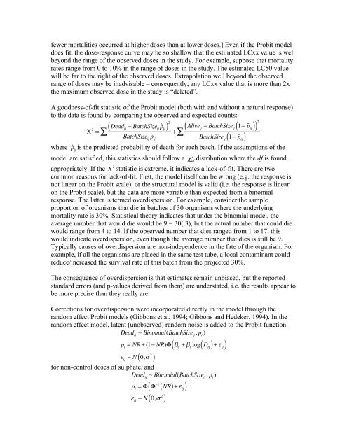
fewer mortalities occurred at higher doses than at lower doses.] Even if the Probit modeldoes fit, the dose-response curve may be so shallow that the estimated LCxx value is wellbeyond the range of the observed doses in the study. For example, suppose that mortalityrates range from 0 to 10% in the range of doses in the study. The estimated LC50 valuewill be far to the right of the observed doses. Extrapolation well beyond the observedrange of doses may be inadvisable – consequently, any LCxx value that is more than 2xthe maximum observed dose in the study is “deleted”.A goodness-of-fit statistic of the Probit model (both with and without a natural response)to the data is found by comparing the observed and expected counts:( Dead! 2 ij" BatchSize ij ˆp ij ) 2( Alive ij" BatchSize ij ( 1" ˆp ij )) 2= # + #BatchSize ij ˆp ijBatchSize ij ( 1" ˆp ij )where ˆp ijis the predicted probability of death for each batch. If the assumptions of themodel are satisfied, this statistics should follow a ! 2dfdistribution where the df is foundappropriately. If the X 2 statistic is extreme, it indicates a lack-of-fit. There are twocommon reasons for lack-of-fit. First, the model itself can be wrong (e.g. the response isnot linear on the Probit scale), or the structural model is valid (i.e. the response is linearon the Probit scale), but the data are more variable than expected from a binomialresponse. The latter is termed overdispersion. For example, consider the sampleproportion of organisms that die in batches of 30 organisms where the underlyingmortality rate is 30%. Statistical theory indicates that under the binomial model, theaverage number that would die would be 9 = 30(.3), but the actual number that could diewould range from 4 to 14. If the observed number that dies ranged from 1 to 17, thiswould indicate overdispersion, even though the average number that dies is still be 9.Typically causes of overdispersion are non-independence in the fate of the organism. Forexample, if all the organisms are placed in the same test tube, a local contaminant couldreduce/increased the survival rate of this batch from the projected 30%.The consequence of overdispersion is that estimates remain unbiased, but the reportedstandard errors (and p-values derived from them) are understated, i.e. the results appear tobe more precise than they really are.Corrections for overdispersion were incorporated directly in the model through therandom effect Probit models (Gibbons et al, 1994; Gibbons and Hedeker, 1994). In therandom effect model, latent (unobserved) random noise is added to the Probit function:Dead ij! Binomial(BatchSize ij, p i)( ( ) + $ ij )p i= NR + (1! NR)" # 0+ # ilog D ij( )$ ij! N 0,% 2for non-control doses of sulphate, andDead ij! Binomial(BatchSize ij, p i)( )( )p i= ! ! "1( NR) + # ij# ij! N 0,$ 2