Drill Down Till You Drop: OLAP Without Windows - NESUG

More documents

Recommendations

Info

discarded since REGION is never selected by drillingdown on CITY).• If we continue this process to the last variable, CITY,we see that the only _TYPE_ values needed are 1, 3,7, 15 and 31. At each of these levels, the subgroupincludes the CLASS variables corresponding to thevariable at that level, plus all variables which havealready been “drilled down on” in the hierarchy.If we only include these types, how much will that reducethe size of the output dataset? That will depend upon thenumber of distinct levels for each _TYPE_. Referring toTable 2, we can see that we are now left with a datasetcontaining only 68 observations, drastically reducing thenumber of observations in the output summary data set,relative to both the original “drill” dataset, and the output“temp” dataset.Table 2_TYPE_ SUBGROUP OBS1 Date 53 Country by Date 107 Region by Country by Date 1515 State by Region by Country by 34Date31 City by State by Region byCountry by Date34We can generalize the above example by stating that in adrill down hierarchy, where we have N CLASS variableswhich have been arranged in drill down order from rightto left, in order to perform a drill down as describedabove, we only require the output observations which have_TYPE_ values in:{ 2 0 ,2 0 + 2 1 ,2 0 + 2 1 + 2 2 ,2 0 + 2 1 + 2 2 + 2 3 ……….. ,2 0 + 2 1 + 2 2 + 2 3 + 2 N-1 }with 0 being the most rightmost position, and increasingby 1 for each variable to the left. (1.1)Using the output data temp as generated above we createthe optimized drill down dataset by subsetting:data temp;set temp;4where _TYPE_ in (1, 3, 7, 15, 31);A special form of the above formula exists when the drillhierarchy starts from the rightmost variable in the CLASSstatement. In this case the first _TYPE_ value is always1, and the next drill down value is generated bymultiplying the last variable by 2 and adding 1. (1.2)In a “drill-up” situation, this would be equivalent tosubtracting 1 from the current level and then dividing by2.If we still are left with a large output data set, afterreducing the size in this manner, we may choose to placean index on the _TYPE_ variable if it will providesignificantly quicker access to the data.PROC SQL;create index _TYPE_ on temp (_TYPE_);Reordering the Drill HierarchyIt is usually best to set up the order of the drill variablesfrom right to left, as we just did in the preceding example,however it is not essential to do so.Let’s say we were interested in reordering the drillhierarchy starting with COUNTRY, and then drillingdown on DATE, REGION, all the way down to CITY.Our drill hierarchy now becomes:COUNTRY→ DATE→ REGION → STATE→ CITYSince we have already created the optimized database,how does that affect the reordering of the variables ? Wecould always reorder the positions of the drill variablesfrom right to left, and rerun the original PROCSUMMARY etc., but there is another way:If we express our modified drill hierarchy with respect topowers of 2 we have:2 1 → 2 0 → 2 2 → 2 3 → 2 4If we examine the exponent of 2 in each case, we see thatit represents the position, starting with 0, of the level inthe CLASS statement.Since COUNTRY is now the 2nd variable from the righton the CLASS statement, it has a _TYPE_ value of 2 1 , or2. This becomes the first _TYPE_ value. The nextvariable in the hierarchy is DATE, which has a _TYPE_value of 1, so we add these two values together to get thenext _TYPE_ value which is 3. The next level isREGION, so we add the _TYPE_ value of 4 to get the
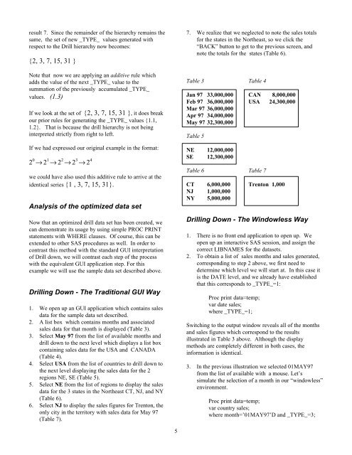
esult 7. Since the remainder of the hierarchy remains thesame, the set of new _TYPE_ values generated withrespect to the Drill hierarchy now becomes:{2, 3, 7, 15, 31 }Note that now we are applying an additive rule whichadds the value of the next _TYPE_ value to thesummation of the previously accumulated _TYPE_values. (1.3)If we look at the set of {2, 3, 7, 15, 31 }, it does breakour prior rules for generating the _TYPE_ values {1.1,1.2}. That is because the drill hierarchy is not beinginterpreted strictly from right to left.If we had expressed our original example in the format:2 0 → 2 1 → 2 2 → 2 3 → 2 4we could have also used this additive rule to arrive at theidentical series {1 , 3, 7, 15, 31}.Analysis of the optimized data setNow that an optimized drill data set has been created, wecan demonstrate its usage by using simple PROC PRINTstatements with WHERE clauses. Of course, this can beextended to other SAS procedures as well. In order tocontrast this method with the standard GUI interpretationof Drill down, we will contrast each step of the processwith the equivalent GUI application step. For thisexample we will use the sample data set described above.Drilling Down - The Traditional GUI Way1. We open up an GUI application which contains salesdata for the sample data set described.2. A list box which contains months and associatedsales data for that month is displayed (Table 3).3. Select May 97 from the list of available months anddrill down to the next level which displays a list boxcontaining sales data for the USA and CANADA(Table 4).4. Select USA from the list of countries to drill down tothe next level displaying the sales data for the 2regions NE, SE (Table 5).5. Select NE from the list of regions to display the salesdata for the 3 states in the Northeast CT, NJ, and NY(Table 6).6. Select NJ to display the sales figures for Trenton, theonly city in the territory with sales data for May 97(Table 7).7. We realize that we neglected to note the sales totalsfor the states in the Northeast, so we click the“BACK” button to get to the previous screen, andnote the totals for the states (Table 6).Table 3 Table 4Jan 97 33,000,000 CAN 8,000,000Feb 97 36,000,000 USA 24,300,000Mar 97 36,000,000Apr 97 34,000,000May 97 32,300,000Table 5NE 12,000,000SE 12,300,000Table 6 Table 7CT 6,000,000 Trenton 1,000NJ 1,000,000NY 5,000,000Drilling Down - The Windowless Way1. There is no front end application to open up. Weopen up an interactive SAS session, and assign thecorrect LIBNAMES for the datasets.2. To obtain a list of sales months and sales generated,corresponding to step 2 above, we first need todetermine which level we will start at. In this case itis the DATE level, and we already have establishedthat this corresponds to _TYPE_=1:Proc print data=temp;var date sales;where _TYPE_=1;Switching to the output window reveals all of the monthsand sales figures which correspond to the resultsillustrated in Table 3 above. Although the displaymethods are completely different in both cases, theinformation is identical.3. In the previous illustration we selected 01MAY97from the list of available with a mouse. Let’ssimulate the selection of a month in our “windowless”environment.Proc print data=temp;var country sales;where month=’01MAY97’D and _TYPE_=3;5
Page 2 and 3: Sample DataA sample demonstration d
Page 6: • The month which is being select
Page 9 and 10: down database has been built, it is

Drill Down Till You Drop: OLAP Without Windows - NESUG

Create successful ePaper yourself

Delete template?

Save as template?