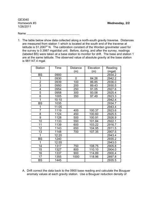
1. The table below show data collected along a

GE3040Homework #3 Wednesday, 2/21/26/2011Name ________________________________1. The table below show data collected along a north-south gravity traverse. Distancesare measured from station 1 which is located at the south end of the traverse atlatitude is 51.2067 o N. The calibration constant of the Worden gravimeter used forthe survey is 0.3987 mgal/dial unit. Before, during, and after the survey, readings(labeled BS) were taken at a base station to monitor for drift. The base and station 1are at the same latitude. The observed value of absolute gravity at the base stationis 981147.4 mgal.Station Time Distance(m)Elevation(m)Reading(mgal)BS 0900 2934.21 0930 0 84.26 2942.22 0939 100 86.85 2936.03 0950 200 89.43 2930.54 0954 250 91.05 2927.65 0958 300 93.08 2925.46 1005 350 97.49 2923.31 10:10 2942.4BS 1035 2934.71 11:05 2943.47 1119 400 100.37 2923.68 1124 450 100.60 2925.59 1128 500 100.91 2926.910 1133 550 101.84 2922.111 1139 600 103.22 2916.712 1143 650 104.95 2911.513 1148 700 107.35 2907.51 12:20 2943.4BS 1240 2935.21 12:55 2943.014 1317 750 108.75 2905.815 1327 800 110.10 2904.016 1337 900 114.89 2900.417 1355 1000 118.96 2897.8BS 1445 2935.5A. Drift correct the data back to the 0900 base reading and calculate the Bougueranomaly values at each gravity station. Use a Bouguer reduction density of

2.70 Mg/m 3 . Use a spreadsheet (a template can be found athttp://www.geo.mtu.edu/~jdiehl/Homework/3040h3s11.xls) to do this if possible.You'll save time in the long run.B. Construct a graph illustrating the variation in topography, observed gravity (useΔg instead of g obs ), and the Bouguer gravity anomaly along the survey line (i.e.,as a function of distance). [Hint: Use a secondary y-axis to plot topographicelevations.] Why does g obs (or Δg) decrease with increasing elevation?C. Using the data from station 1, determine the probable error associated withreading the gravimeter, i.e. calculate the standard error of the mean (S e = σ/√n;where σ 2 = [Σ n j=1 (X j - μ) 2 ]/n; μ is the mean; and n is the number of observations).Comment on this value.D. Create a separate plot of the Bouguer Anomaly vs. distance and on that plotdraw in the regional gravity field for the Bouguer gravity anomaly. Now subtractthe regional field from the Bouguer gravity anomaly and plot the residual.2. Use the terrain correction table from the handouts to calculate the terrain correctionfor Zones G and H (in mgals) for the gravity station (elevation = 1119 feet) located atthe center of the template shown on the next page. Create a table showing theaverage elevation, elevation difference, and the terrain correction for each of thetwelve numbered sectors of Zones G and H. Now sum the terrain correction valuesfor the twelve sectors of G and H. This is the terrain correction for each zone. Whatare they? Contour interval is 20 feet.3. Using the attached Bouguer anomaly map (contour interval 50 gu) do the following:a. Draw in what you consider to be the regional field on the map using smoothedcontour approach (assume a planar regional) and then subtract this regional fromthe observed field (i.e., at points where the observed and regional intersect).Now contour the residual anomaly using a 50 gu contour interval. Use tracingpaper to do this. Be sure to label contours.b. Now using the same map construct the Bouguer gravity profile along line A-A'(shown on map). Again draw in the regional gravity field (smoothed profile) andsubtract this regional from the observed gravity values and plot the residualanomaly.