Hydromagnetic waves in Earth's core and their influence on ...
Hydromagnetic waves in Earth's core and their influence on ...
Hydromagnetic waves in Earth's core and their influence on ...

You also want an ePaper? Increase the reach of your titles
YUMPU automatically turns print PDFs into web optimized ePapers that Google loves.
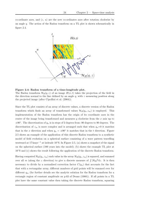
24 Chapter 2 — Space-time analysisco-ord<str<strong>on</strong>g>in</str<strong>on</strong>g>ate axes, <str<strong>on</strong>g>and</str<strong>on</strong>g> (z, u) are the new co-ord<str<strong>on</strong>g>in</str<strong>on</strong>g>ates axes after rotati<strong>on</strong> clockwise byan angle q. The acti<strong>on</strong> of the Rad<strong>on</strong> transform <strong>on</strong> a TL plot is shown schematically <str<strong>on</strong>g>in</str<strong>on</strong>g>figure 2.4.−Figure 2.4: Rad<strong>on</strong> transform of a time-l<strong>on</strong>gitude plot.The Rad<strong>on</strong> transform H R (q, z) of an image H(x, t) takes the projecti<strong>on</strong> of the field <str<strong>on</strong>g>in</str<strong>on</strong>g>the directi<strong>on</strong> normal to the l<str<strong>on</strong>g>in</str<strong>on</strong>g>e def<str<strong>on</strong>g>in</str<strong>on</strong>g>ed by an angle q, with z measur<str<strong>on</strong>g>in</str<strong>on</strong>g>g positi<strong>on</strong> al<strong>on</strong>gthe projected image (after Cipoll<str<strong>on</strong>g>in</str<strong>on</strong>g>i et al. (2004)).S<str<strong>on</strong>g>in</str<strong>on</strong>g>ce the TL plot c<strong>on</strong>sists of an array of discrete values, a discrete versi<strong>on</strong> of the Rad<strong>on</strong>transform which f<str<strong>on</strong>g>in</str<strong>on</strong>g>ds an array of transformed values H R (q n , z m ) is employed. Thisimplementati<strong>on</strong> of the Rad<strong>on</strong> transform has the orig<str<strong>on</strong>g>in</str<strong>on</strong>g> of its coord<str<strong>on</strong>g>in</str<strong>on</strong>g>ate axes <str<strong>on</strong>g>in</str<strong>on</strong>g> thecentre of the image be<str<strong>on</strong>g>in</str<strong>on</strong>g>g transformed <str<strong>on</strong>g>and</str<strong>on</strong>g> measures q clockwise from the x axis up to±90 ◦ . The discretisati<strong>on</strong> of q n is <str<strong>on</strong>g>in</str<strong>on</strong>g> steps of 2 degrees from -90 degrees to 90 degrees. Thediscretisati<strong>on</strong> of z m is more complex <str<strong>on</strong>g>and</str<strong>on</strong>g> is arranged such that when q n =0 it matchesthat <str<strong>on</strong>g>in</str<strong>on</strong>g> the x directi<strong>on</strong> <str<strong>on</strong>g>and</str<strong>on</strong>g> when q n = ±90 ◦ it matches that <str<strong>on</strong>g>in</str<strong>on</strong>g> the t directi<strong>on</strong>. Figure2.5 shows an example of the applicati<strong>on</strong> of this discrete Rad<strong>on</strong> transform to a syntheticmodel of field evoluti<strong>on</strong> <strong>on</strong> a spherical surface c<strong>on</strong>sist<str<strong>on</strong>g>in</str<strong>on</strong>g>g of a wave pattern travell<str<strong>on</strong>g>in</str<strong>on</strong>g>gwestward at 17 kmyr −1 at latitude 10 ◦ S. In Figure 2.5, (a) shows a snapshot of the signal<strong>on</strong> the spherical surface (100 years <str<strong>on</strong>g>in</str<strong>on</strong>g>to the model); (b) shows the example TL plot at10 ◦ S <str<strong>on</strong>g>and</str<strong>on</strong>g> (c) shows the result follow<str<strong>on</strong>g>in</str<strong>on</strong>g>g the applicati<strong>on</strong> of the discrete Rad<strong>on</strong> transform.Hav<str<strong>on</strong>g>in</str<strong>on</strong>g>g computed H R (q n , z m ) each value <str<strong>on</strong>g>in</str<strong>on</strong>g> the array H R (q n , z m ) is squared, <str<strong>on</strong>g>and</str<strong>on</strong>g> summedover all m (al<strong>on</strong>g the z directi<strong>on</strong>) to give a discrete measure of ∫ |H R | 2 dz. It is thennecessary to divide by a normalised correcti<strong>on</strong> factor C(q n ) that accounts for the factthat with a rectangular array, different numbers of grid po<str<strong>on</strong>g>in</str<strong>on</strong>g>ts will be summed over fordifferent q m (for further details see the analytic soluti<strong>on</strong> for the Rad<strong>on</strong> transform for arectangle regi<strong>on</strong> of c<strong>on</strong>stant amplitude <strong>on</strong> p.63 of Deans (1988)). If all po<str<strong>on</strong>g>in</str<strong>on</strong>g>ts <str<strong>on</strong>g>in</str<strong>on</strong>g> a TLplot have the same c<strong>on</strong>stant value then tak<str<strong>on</strong>g>in</str<strong>on</strong>g>g the discrete Rad<strong>on</strong> transform, squar<str<strong>on</strong>g>in</str<strong>on</strong>g>g