Construction of Iso-contours, Bisectors and Voronoi Diagrams on ...

More documents

Recommendations

Info

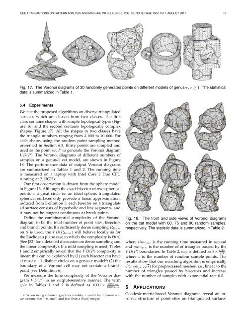
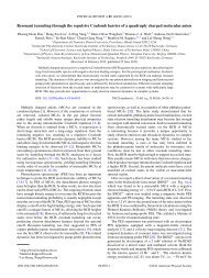
IEEE TRANSACTIONS ON PATTERN ANALYSIS AND MACHINE INTELLIGENCE, VOL. 33, NO. 8, PAGE 1502-1517, AUGUST 2011 10Fig. 17. The <strong>Voronoi</strong> diagrams <strong>of</strong> 30 r<strong>and</strong>omly generated points on different models <strong>of</strong> genus-r, r ≥ 1. The statisticaldata is summarized in Table 1.5.4 ExperimentsWe test the proposed algorithms on diverse triangulatedsurfaces which are chosen from two classes. The firstclass contains shapes with simple topological types (Figure16) <strong>and</strong> the second contains topologically complexshapes (Figure 17). All the shapes in two classes havethe triangle numbers ranging from 3, 000 to 10, 000. Foreach shape, using the r<strong>and</strong>om point sampling methodpresented in Section 6.3, thirty points are sampled <strong>and</strong>used as the point set P to generate the <strong>Voronoi</strong> diagramV D(P ). The <strong>Voronoi</strong> diagrams <strong>of</strong> different numbers <strong>of</strong>samples on a genus-1 cat model, are shown in Figure18. The performance data <strong>of</strong> output <strong>Voronoi</strong> diagramsare summarized in Tables 1 <strong>and</strong> 2. The running timeis measured on a laptop with Intel Core 2 Duo CPUrunning at 2.13GHz.Our first observation is drawn from the sphere modelin Figure 16. Although the exact bisector <strong>of</strong> two sphericalpoints is a great circle on an ideal sphere, triangulatedspherical surfaces only provide a linear approximation:induced from Definition 5, each bisector on a triangulatedsurface consists <strong>of</strong> hyperbolic <strong>and</strong> line segments, <strong>and</strong>it may not be tangent continuous at break points.Define the combinatorial complexity <strong>of</strong> the <strong>Voronoi</strong>diagram to be the total number <strong>of</strong> point sites, bisectors<strong>and</strong> branch points. If a sufficiently dense sampling P denseon S is used, the V D(P dense ) will behave locally as forthe Euclidean plane case in which the complexity is Θ(n)(See [52] for a detailed discussion on dense sampling <strong>and</strong>the linear complexity). If a mild sampling is used, Tables1 <strong>and</strong> 2 empirically reveal that the V D(P ) complexity islinear: this can be explained by (1) each bisector can haveat most r + 1 distinct circles on a genus-r model 2 ; (2) theboundary <strong>of</strong> a <strong>Voronoi</strong> cell may not contain a branchpoint (see Definition 6).We measure the time complexity <strong>of</strong> the <strong>Voronoi</strong> diagramV D(P ) in an output-sensitive manner. The termcplx in Tables 1 <strong>and</strong> 2 is defined as 1000 × time secnum ptri,2. When using different graphics models, r could be different <strong>and</strong>we assume that r is small <strong>and</strong> less than a fixed integer.Fig. 18. The front <strong>and</strong> side views <strong>of</strong> <strong>Voronoi</strong> diagramson the cat model with 60, 75 <strong>and</strong> 90 r<strong>and</strong>om samples,respectively. The statistic data is summarized in Table 2.where time sec is the running time measured in second<strong>and</strong> num ptri is the number <strong>of</strong> <strong>of</strong> triangles passed by theV D(P ) boundaries. In Table 2, exp is defined as 8 × cplx √ s,where s is the number <strong>of</strong> r<strong>and</strong>om sample points. Theresults show√that our marching algorithm is empiricallyO(num ptri s) for preprocessed meshes, i.e., linear to thenumber <strong>of</strong> triangles passed by bisectors <strong>and</strong> increasewith the number <strong>of</strong> samples with exponential rate 0.5.6 APPLICATIONSGeodesic-metric-based <strong>Voronoi</strong> diagrams reveal an intrinsicstructure <strong>of</strong> point sites on triangulated surfaces
IEEE TRANSACTIONS ON PATTERN ANALYSIS AND MACHINE INTELLIGENCE, VOL. 33, NO. 8, PAGE 1502-1517, AUGUST 2011 11model tri no bh pt bs no bk pt time(sec) cplxsphere 4,074 54 81 558 11.9 + 0.55 0.574shark 3,412 53 81 523 14.47 + 0.98 0.592tooth 5,036 50 75 648 20.31 + 0.57 0.604penguin 4,416 56 84 613 17.6 + 0.61 0.596dinosaur 3,433 48 74 570 11.68 + 0.48 0.556horse 3,212 52 80 497 9.89 + 0.48 0.606sharp 4,680 50 78 642 20.11 + 0.54 0.548tri-dome 7,824 72 108 1,141 42.25 + 1.17 0.679cat 10,960 58 87 1,117 55.67 + 0.98 0.611cup 8,400 62 93 1,034 52.37 + 0.95 0.632part 4,272 68 102 626 14.73 + 0.70 0.651TABLE 1The complexity (number <strong>of</strong> triangles, branch points,bisectors, break points <strong>and</strong> time in seconds) <strong>of</strong> the<strong>Voronoi</strong> diagrams on diverse shapes, shown in Figures16 <strong>and</strong> 17. The time is measured in two parts, fordistance field construction <strong>and</strong> <strong>Voronoi</strong> diagramconstruction, respectively. See Sec. 5.4 for cplx.samples branch pt bisector no break pt cplx exp15 28 42 851 0.436 0.90130 58 87 1,117 0.614 0.89745 90 135 1,265 0.793 0.94560 118 177 1,449 0.96 0.99175 148 222 1,576 1.117 1.03290 174 261 1,705 1.196 1.009TABLE 2The complexity <strong>of</strong> the <strong>Voronoi</strong> diagrams on the cat modelshown in Figure 18, with different sample points. SeeSec. 5.4 for exp.M. Below we present three applications that show thepower <strong>of</strong> the <strong>Voronoi</strong> diagrams on M as a basic tool inpattern analysis.6.1 Geodesic RemeshingNowadays 3D reconstruction from range data <strong>of</strong>ten producesdense triangle meshes with non-uniform triangleaspect ratio [16]. For many applications, partial differentialequations need to be solved on these triangulatedsurfaces M [57]. To achieve better numerical precision,it is <strong>of</strong>ten required to remesh M into M ′ such that thetriangles in M ′ are as close as possible to equilateraltriangles.To uniformly sample the surface M, farthest pointsamples are used [15], [47]. Given a set <strong>of</strong> samplesP = {p 1 , p 2 , · · · , p m } on M, we define the dispersion inP byδ(P ) = sup{minD p(x)}x∈S p∈Pwhere D p (x) is the geodesic distance between p <strong>and</strong> x. T<strong>of</strong>ind a new sample p m+1 that minimizes the dispersionδ(P ∪ p m+1 ), the position <strong>of</strong> p m+1 must be at one <strong>of</strong> thebranch points <strong>of</strong> V D(P ) or lie on the bisector whichdoes not end at branch points. This property dramaticallyreduces the search space in M. Starting from anarbitrary sample, more samples are added one by oneFig. 19. Geodesic remesh <strong>of</strong> a tooth model. The first rowshows two views <strong>of</strong> uniform samplings (red points) on anoriginal mesh. The second row shows the remesh withthe uniform samples.by incrementally updating the <strong>Voronoi</strong> diagram. Leibon<strong>and</strong> Letscher [36] show that if the samples are sufficientlydense, the dual triangulation <strong>of</strong> the <strong>Voronoi</strong> diagram onM exists <strong>and</strong> thus <strong>of</strong>fers us a solution to the geodesicremeshing problem. An example is shown in Figure 19.Peyre <strong>and</strong> Cohen [54] presented an approach similar toours, but used an approximate geodesic metric which iscomputed by Kimmel <strong>and</strong> Sethian’s fast marching algorithm[29]. Since the original meshes can have extremelyslivered triangles before remeshing, the numerical fastmarching methods might be contaminated by numericalerrors, while our method is more accurate <strong>and</strong> robust 3since we use the exact geodesic metric.6.2 Tree Skeleton Extraction <strong>and</strong> ClassificationSkeletons <strong>of</strong> 3D articulated models reveal rich topologicalinformation <strong>and</strong> play an important role in patternrecognition <strong>and</strong> computer animation. Many elegantmathematical tools have been investigated for extractingskeletons from 3D models, including medial axis, shockgraphs, Reeb graphs with Morse functions, etc [17], [58].Despite the novelties in these tools, the resulting skeletonsdo not take the full advantage <strong>of</strong> vision perception<strong>and</strong> are not visually simple. E.g., mixed 1D <strong>and</strong> 2D celltypes appear in the medial axis/surface <strong>of</strong> 3D objects<strong>and</strong> are sensitive to tiny noises on surfaces [20].Observing that the human vision system is able toinfer visually simple skeletons with full functionality,3. To robustly h<strong>and</strong>le the degenerate cases arisen in numericalcomputation <strong>of</strong> our constructive algorithms, we use the toolkit proposedin [39], which classifies <strong>and</strong> h<strong>and</strong>les degeneracies in two types:degeneracies on geometric intersection <strong>and</strong> degeneracies on geodesicdiscontinuities.
Page 4 and 5: IEEE TRANSACTIONS ON PATTERN ANALYS
Page 14: IEEE TRANSACTIONS ON PATTERN ANALYS

Construction of Iso-contours, Bisectors and Voronoi Diagrams on ...

Create successful ePaper yourself

Delete template?

Save as template?