author's proof

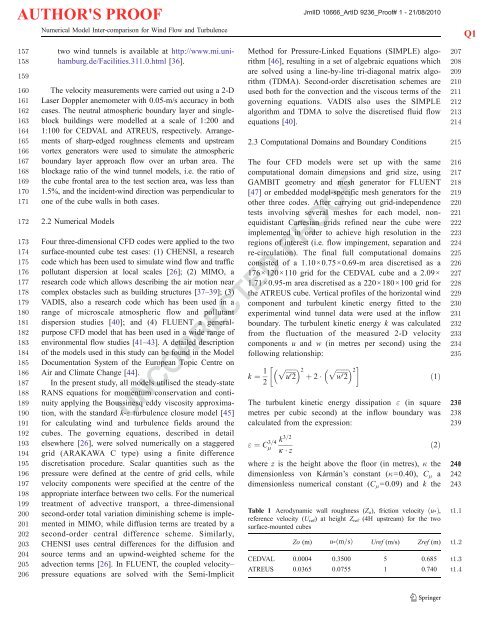
AUTHOR'S PROOFNumerical Model Inter-comparison for Wind Flow and TurbulenceJrnlID 10666_ArtID 9236_Proof# 1 - 21/08/2010Q1157 two wind tunnels is available at http://www.mi.uni-158 hamburg.de/Facilities.311.0.html [36].159160 The velocity measurements were carried out using a 2-D161 Laser Doppler anemometer with 0.05-m/s accuracy in both162 cases. The neutral atmospheric boundary layer and single-163 block buildings were modelled at a scale of 1:200 and164 1:100 for CEDVAL and ATREUS, respectively. Arrange-165 ments of sharp-edged roughness elements and upstream166 vortex generators were used to simulate the atmospheric167 boundary layer approach flow over an urban area. The168 blockage ratio of the wind tunnel models, i.e. the ratio of169 the cube frontal area to the test section area, was less than170 1.5%, and the incident-wind direction was perpendicular to171 one of the cube walls in both cases.172 2.2 Numerical Models173 Four three-dimensional CFD codes were applied to the two174 surface-mounted cube test cases: (1) CHENSI, a research175 code which has been used to simulate wind flow and traffic176 pollutant dispersion at local scales [26]; (2) MIMO, a177 research code which allows describing the air motion near178 complex obstacles such as building structures [37–39]; (3)179 VADIS, also a research code which has been used in a180 range of microscale atmospheric flow and pollutant181 dispersion studies [40]; and (4) FLUENT a general-182 purpose CFD model that has been used in a wide range of183 environmental flow studies [41–43]. A detailed description184 of the models used in this study can be found in the Model185 Documentation System of the European Topic Centre on186 Air and Climate Change [44].187 In the present study, all models utilised the steady-state188 RANS equations for momentum conservation and conti-189 nuity applying the Boussinesq eddy viscosity approxima-190 tion, with the standard k-ε turbulence closure model [45]191 for calculating wind and turbulence fields around the192 cubes. The governing equations, described in detail193 elsewhere [26], were solved numerically on a staggered194 grid (ARAKAWA C type) using a finite difference195 discretisation procedure. Scalar quantities such as the196 pressure were defined at the centre of grid cells, while197 velocity components were specified at the centre of the198 appropriate interface between two cells. For the numerical199 treatment of advective transport, a three-dimensional200 second-order total variation diminishing scheme is imple-201 mented in MIMO, while diffusion terms are treated by a202 second-order central difference scheme. Similarly,203 CHENSI uses central differences for the diffusion and204 source terms and an upwind-weighted scheme for the205 advection terms [26]. In FLUENT, the coupled velocity–206 pressure equations are solved with the Semi-ImplicitMethod for Pressure-Linked Equations (SIMPLE) algorithm[46], resulting in a set of algebraic equations whichare solved using a line-by-line tri-diagonal matrix algorithm(TDMA). Second-order discretisation schemes areused both for the convection and the viscous terms of thegoverning equations. VADIS also uses the SIMPLEalgorithm and TDMA to solve the discretised fluid flowequations [40].2.3 Computational Domains and Boundary ConditionsThe four CFD models were set up with the samecomputational domain dimensions and grid size, usingGAMBIT geometry and mesh generator for FLUENT[47] or embedded model-specific mesh generators for theother three codes. After carrying out grid-independencetests involving several meshes for each model, nonequidistantCartesian grids refined near the cube wereimplemented in order to achieve high resolution in theregions of interest (i.e. flow impingement, separation andre-circulation). The final full computational domainsconsisted of a 1.10×0.75×0.69-m area discretised as a176×120×110 grid for the CEDVAL cube and a 2.09×1.71×0.95-m area discretised as a 220×180×100 grid forthe ATREUS cube. Vertical profiles of the horizontal windcomponent and turbulent kinetic energy fitted to theexperimental wind tunnel data were used at the inflowboundary. The turbulent kinetic energy k was calculatedfrom the fluctuation of the measured 2-D velocitycomponents u and w (in metres per second) using thefollowing relationship:k ¼ 1 pffiffiffiffiffiffi 2 pffiffiffiffiffiffiffi 2u20 2 þ 2 w 0 2ð1ÞThe turbulent kinetic energy dissipation ε (in squaremetres per cubic second) at the inflow boundary wascalculated from the expression:UNCORRECTED PROOF" ¼ C 3=4mk 3=2k zð2Þwhere z is the height above the floor (in metres), κ thedimensionless von Kármán’s constant (κ=0.40), C μ adimensionless numerical constant (C μ =0.09) and k theTable 1 Aerodynamic wall roughness (Z o ), friction velocity ðu»Þ,reference velocity (U ref ) at height Z ref (4H upstream) for the twosurface-mounted cubesZo (m)u» ðm=sÞ Uref (m/s) Zref (m)CEDVAL 0.0004 0.3500 5 0.685ATREUS 0.0365 0.0755 1 0.740207208209210211212213214215216217218219220221222223224225226227228229230231232233234235236 237238239240 241242243t1.1t1.2t1.3t1.4