2 Physical Properties of Marine Sediments - Blogs Unpad

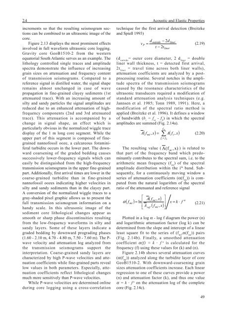
2.4 Acoustic and Elastic Propertiesincrements so that the resulting seismogram sectionscan be combined to an ultrasonic image of thecore.Figure 2.13 displays the most prominent effectsinvolved in full waveform ultrasonic core logging.Gravity core GeoB1510-2 from the westernequatorial South Atlantic serves as an example. Thelithology controlled single traces and amplitudespectra demonstrate the influence of increasinggrain sizes on attenuation and frequency contentof transmission seismograms. Compared to areference signal in distilled water, the signal shaperemains almost unchanged in case of wavepropagation in fine-grained clayey sediments (1stattenuated trace). With an increasing amount ofsilty and sandy particles the signal amplitudes arereduced due to an enhanced attenuation of highfrequencycomponents (2nd and 3rd attenuatedtrace). This attenuation is accompanied by achange in signal shape, an effect which isparticularly obvious in the normalized wiggle tracedisplay of the 1 m long core segment. While theupper part of this segment is composed of finegrainednannofossil ooze, a calcareous foraminiferalturbidite occurs in the lower part. The downwardcoarsening of the graded bedding causessuccessively lower-frequency signals which caneasily be distinguished from the high-frequencytransmission seismograms in the upper fine-grainedpart. Additionally, first arrival times are lower in thecoarse-grained turbidite than in fine-grainednannofossil oozes indicating higher velocities insilty and sandy sediments than in the clayey part.A conversion of the normalized wiggle traces to agray-shaded pixel graphic allows us to present thefull transmission seismogram information on ahandy scale. In this ultrasonic image of thesediment core lithological changes appear assmooth or sharp phase discontinuities resultingfrom the low-frequency waveforms in silty andsandy layers. Some of these layers indicate agraded bedding by downward prograding phases(1.60 - 2.10 m, 4.70 - 4.80 m, 7.50 - 7.60 m). The P-wave velocity and attenuation log analyzed fromthe transmission seismograms support theinterpretation. Coarse-grained sandy layers arecharacterized by high P-wave velocities and attenuationcoefficients while fine-grained parts reveallow values in both parameters. Especially, attenuationcoefficients reflect lithological changesmuch more sensitively than P-wave velocities.While P-wave velocities are determined onlineduring core logging using a cross-correlationtechnique for the first arrival detection (Breitzkeand Spieß 1993)vPd outside − 2dliner= (2.19)t − 2tliner(d outside= outer core diameter, 2 d liner= doubleliner wall thickness, t = detected first arrival,2t liner= travel time across both liner walls),attenuation coefficients are analyzed by a postprocessingroutine. Several notches in the amplitudespectra of the transmission seismogramscaused by the resonance characteristics of theultrasonic transducers required a modification ofstandard attenuation analysis techniques (e.g.Jannsen et al. 1985; Tonn 1989, 1991). Here, amodification of the spectral ratio method isapplied (Breitzke et al. 1996). It defines a windowof bandwidth (b i= f ui- f li) in which the spectralamplitudes are summed (Fig. 2.14a).∑( f x) A( f x)mifA , , (2.20)= ui fi= fliThe resulting value ( Af (mi, x)) is related tothat part of the frequency band which predominantlycontributes to the spectral sum, i.e. to thearithmetic mean frequency (f mi) of the spectralamplitude distribution within the i th band. Subsequently,for a continuously moving window aseries of attenuation coefficients (α(f mi)) is computedfrom the natural logarithm of the spectralratio of the attenuated and reference signal( f )⎡⎢⎣A( f mi , x)( f , x)⎤⎥⎦nα mi = lnx = k ⋅ f (2.21)⎢ Arefmi⎥Plotted in a log α - log f diagram the power (n)and logarithmic attenuation factor (log k) can bedetermined from the slope and intercept of a linearleast square fit to the series of (f mi,α(f mi)) pairs(Fig. 2.14b). Finally, a smoothed attenuationcoefficient α(f) = k ⋅ f n is calculated for thefrequency (f) using these values for (k) and (n).Figure 2.14b shows several attenuation curves(α(f mi)) analyzed along the turbidite layer of coreGeoB1510-2. With downward-coarsening grainsizes attenuation coefficients increase. Each linearregression to one of these curves provide a power(n) and attenuation factor (k), and thus one valueα = k ⋅ f n on the attenuation log of the completecore (Fig. 2.14c).i49