RENDICONTI DEL SEMINARIO MATEMATICO

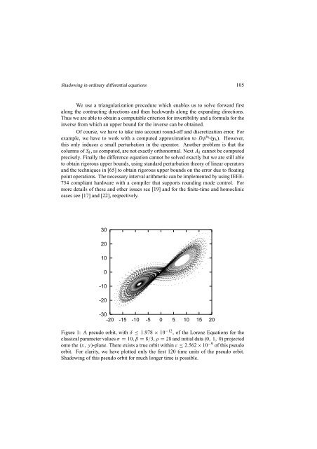
Shadowing in ordinary differential equations 105We use a triangularization procedure which enables us to solve forward firstalong the contracting directions and then backwards along the expanding directions.Thus we are able to obtain a computable criterion for invertibility and a formula for theinverse from which an upper bound for the inverse can be obtained.Of course, we have to take into account round-off and discretization error. Forexample, we have to work with a computed approximation to Dφ h k(y k ). However,this only induces a small perturbation in the operator. Another problem is that thecolumns of S k , as computed, are not exactly orthonormal. Next A k cannot be computedprecisely. Finally the difference equation cannot be solved exactly but we are still ableto obtain rigorous upper bounds, using standard perturbation theory of linear operatorsand the techniques in [65] to obtain rigorous upper bounds on the error due to floatingpoint operations. The necessary interval arithmetic can be implemented by using IEEE-754 compliant hardware with a compiler that supports rounding mode control. Formore details of these and other issues see [19] and for the finite-time and homocliniccases see [17] and [22], respectively.3020100-10-20-30-20 -15 -10 -5 0 5 10 15 20Figure 1: A pseudo orbit, with δ ≤ 1.978 × 10 −12 , of the Lorenz Equations for theclassical parameter values σ = 10, β = 8/3, ρ = 28 and initial data (0, 1, 0) projectedonto the (x, y)-plane. There exists a true orbit within ε ≤ 2.562×10 −9 of this pseudoorbit. For clarity, we have plotted only the first 120 time units of the pseudo orbit.Shadowing of this pseudo orbit for much longer time is possible.