RENDICONTI DEL SEMINARIO MATEMATICO

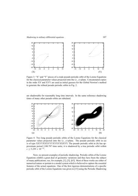
Shadowing in ordinary differential equations 10720151050-5-10-15-20-15 -10 -5 0 5 10 15(X)20151050-5-10-15-20-15 -10 -5 0 5 10 15(Y)Figure 3: “X” and “Y” pieces of a crude pseudo periodic orbit of the Lorenz Equationsfor the classical parameter values projected onto the (x, y)-plane. Concatenated copiesin the order XY and XYY are used as initial guesses for the Global Newton’s methodto generate the refined pseudo periodic orbits in Fig. 2.are shadowable for reasonably long time intervals. In the same reference shadowingtimes of many other pseudo orbits are tabulated.2520151050-5-10-15-20-25-20 -15 -10 -5 0 5 10 15 20(a)3020100-10-20-30-20 -15 -10 -5 0 5 10 15 20(b)Figure 4: Two long pseudo periodic orbits of the Lorenz Equations for the classicalparameter values projected onto the (x, y)-plane. The pseudo periodic orbit in (a)is of type XXYYXXXYYYXYXYXXXYY. The pseudo periodic orbit in (b) has approximateperiod 1100.787 time units; it is shadowed by a true periodic orbit withinε ≤ 5.239 × 10 −12 .Next, we present examples of periodic shadowing. Periodic orbits of the LorenzEquations exhibit a great deal of geometric variations and they have been the subjectof many publications; see, for example, [1], [5], [63]. Most of these works are either ofnumerical nature or pertain to a model system which is believed to capture the essentialfeatures of the actual equations. One of the first rigorous demonstrations of a specificperiodic orbit of the Lorenz Equations was given in [15] using the Periodic Shadowing