RENDICONTI DEL SEMINARIO MATEMATICO

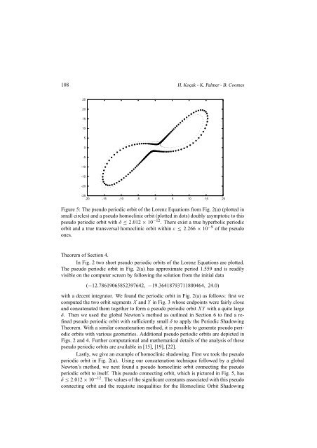
108 H. Koçak - K. Palmer - B. Coomes2520151050-5-10-15-20-25-20 -15 -10 -5 0 5 10 15 20Figure 5: The pseudo periodic orbit of the Lorenz Equations from Fig. 2(a) (plotted insmall circles) and a pseudo homoclinic orbit (plotted in dots) doubly asymptotic to thispseudo periodic orbit with δ ≤ 2.012 × 10 −12 . There exist a true hyperbolic periodicorbit and a true transversal homoclinic orbit within ε ≤ 2.266 × 10 −9 of the pseudoones.Theorem of Section 4.In Fig. 2 two short pseudo periodic orbits of the Lorenz Equations are plotted.The pseudo periodic orbit in Fig. 2(a) has approximate period 1.559 and is readilyvisible on the computer screen by following the solution from the initial data(−12.78619065852397642, −19.36418793711800464, 24.0)with a decent integrator. We found the periodic orbit in Fig. 2(a) as follows: first wecomputed the two orbit segments X and Y in Fig. 3 whose endpoints were fairly closeand concatenated them together to form a pseudo periodic orbit XY with a quite largeδ. Then we used the global Newton’s method as outlined in Section 6 to find a refinedpseudo periodic orbit with sufficiently small δ to apply the Periodic ShadowingTheorem. With a similar concatenation method, it is possible to generate pseudo periodicorbits with various geometries. Additional pseudo periodic orbits are depicted inFigs. 2 and 4. Further computational and mathematical details of the analysis of thesepseudo periodic orbits are available in [15], [19], [22].Lastly, we give an example of homoclinic shadowing. First we took the pseudoperiodic orbit in Fig. 2(a). Using our concatenation technique followed by a globalNewton’s method, we next found a pseudo homoclinic orbit connecting the pseudoperiodic orbit to itself. This pseudo connecting orbit, which is pictured in Fig. 5, hasδ ≤ 2.012 × 10 −12 . The values of the significant constants associated with this pseudoconnecting orbit and the requisite inequalities for the Homoclinic Orbit Shadowing