Modeling drawdowns and drawups in financial markets - Risk.net

58
Beatriz Vaz de Melo Mendes and Vinicius Ratton Brandi
( ) ↑
⎧ yγ
−1
ξ
⎪
1− 1+
ξ , if ξ 0
ψ
G( γ, ξ, ψ;
y)
= ⎨
yγ
⎪ −
ψ
⎩⎪
1−
e , if ξ=0
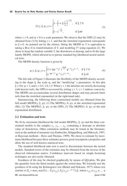
where γ > 0, and ψ > 0 is a scale parameter. We observe that the GPD (2) may be
obtained from (3) by letting γ = 1, and that the stretched exponential corresponds
to ξ = 0. As pointed out by the referee, fitting the MGPD to Y is equivalent to
taking a Box–Cox transformation of Y, and modeling Y γ using equation (2). We
chose to keep the random variable Y, the drawdown or drawup, and to fit the large
family MGPD, which allowed us to pursue standard log-likelihood nested statistical
tests.
The MGPD density function is given by
−1− ξ
⎧
⎪
g( γ, ξ, ψ;
y)
( ξψ yγ ξ ) ψ γ yγ
=
1+ −1 −1 −1,
if ξ ↑ 0
⎨
e− ψ−1y γ
ψ−1γ γ −1
⎩⎪
y ξ
( ) , if =0
The left side of Figure 2 illustrates the flexibility of the MGPD density according
to the shape ξ, the scale ψ, and the “modifying” γ parameters. In this plot
ξ = 0.6, ψ = 3, and γ = 0.5, 1.0, 1.5. When γ < 1 the densities are strictly decreasing
with heavier tails; the GPD is recovered by setting γ = 1; γ > 1 induces concavity.
The MGPD can accommodate several distribution shapes and may present fatter
tails than the stretched exponential (at the right-hand side).
Summarizing, the following three constrained models are obtained from the
full model MGPD(γ, ξ, ψ): (1) The MGPD(γ, 0, ψ), or the stretched exponential
(SE); (2) The MGPD(1, ξ, ψ), or the GPD; (3) The MGPD(1, 0, ψ), or the unit
exponential distribution.
2.2 Estimation and tests
We fit by maximum likelihood the full model MGPD(γ, ξ, ψ) and the three constrained
models to the samples y 1 , y 2 ,…, y n , containing n drawups or absolute
value of drawdowns. Other estimation methods may be found in the literature,
such as the method of moments (see Embrechts, Klüppelberg, and Mikosch, 1997,
or Bayesian methods – Reiss and Thomas, 1999). We chose to estimate by maximum
likelihood because these estimates possess good (asymptotic) properties and
allow the use of well-known statistical tests.
The standard likelihood ratio test is used to discriminate between the nested
models. Standard errors of the estimates may be obtained from the inverse of the
observed information matrix. Confidence intervals based on simple bootstrap
techniques are also easily obtained.
Goodness of fits may be checked graphically by means of QQ-plots. We plot
the quantiles from the fitted models against the sorted data. We formally test the
goodness of fit using the Kolmogorov test (Bickel and Doksum, 1977) whose test
statistic is D n = max i max{i⁄n – F 0 (y (i) ), F 0 (y (i) ) – (i–1) ⁄n}, where y (1) ≤ y (2) ≤ … ≤
URL: www.thejournalofrisk.com Journal of Risk
(3)
(4)