Modeling drawdowns and drawups in financial markets - Risk.net
Modeling drawdowns and drawups in financial markets - Risk.net
Modeling drawdowns and drawups in financial markets - Risk.net

Create successful ePaper yourself
Turn your PDF publications into a flip-book with our unique Google optimized e-Paper software.
<strong>Model<strong>in</strong>g</strong> <strong>drawdowns</strong> <strong>and</strong> <strong>drawups</strong> <strong>in</strong><br />
f<strong>in</strong>ancial <strong>markets</strong><br />
Beatriz Vaz de Melo Mendes<br />
Statistics Department/IM-COPPEAD, Federal University at Rio de Janeiro, RJ, Brazil<br />
V<strong>in</strong>icius Ratton Br<strong>and</strong>i<br />
COPPEAD, Federal University at Rio de Janeiro, RJ, Brazil<br />
Periods of turbulence are often characterized by observed consecutive drops<br />
<strong>in</strong> prices, called “<strong>drawdowns</strong>”. In such cases, static, one-period measures of<br />
risk <strong>in</strong>sufficiently describe downside risk. In this paper, we assess risk by formally<br />
model<strong>in</strong>g these r<strong>and</strong>om str<strong>in</strong>gs of negative returns. We use long-tailed<br />
distributions from extreme value theory to model the severity <strong>and</strong> duration<br />
of the <strong>drawdowns</strong>. This leads to the concept of drawdown-at-risk (DAR) <strong>and</strong><br />
conditional DAR. The proposed distributions adjust properly to extreme values<br />
previously found to be outliers. The paper illustrates the importance of these<br />
concepts with stock market <strong>in</strong>dices.<br />
1 Introduction<br />
Periods of turbulence are often characterized by observed consecutive drops <strong>in</strong><br />
prices, called “<strong>drawdowns</strong>”. Accord<strong>in</strong>g to M<strong>and</strong>elbrot (1963), for daily changes of<br />
stock prices with <strong>in</strong>f<strong>in</strong>ite second moment, the total price change over the span of<br />
the data is usually concentrated <strong>in</strong> a few hectic runs of trad<strong>in</strong>g days. As noticed by<br />
traders <strong>and</strong> <strong>in</strong>vestors, <strong>in</strong> that case, static, one-period measures of risk quite often<br />
fail to fully describe downside risk. 1<br />
Many return distributions have <strong>in</strong>f<strong>in</strong>ite second moment, <strong>and</strong> theoretical<br />
research <strong>in</strong> this area has led to the concept of distributions with fractional dimensions.<br />
2 The study of multifractal trad<strong>in</strong>g time was first <strong>in</strong>troduced by M<strong>and</strong>elbrot<br />
(1972) <strong>in</strong> the context of model<strong>in</strong>g phenomena show<strong>in</strong>g <strong>in</strong>termittent turbulence.<br />
His work was motivated by the observation that the time <strong>in</strong>terval between successive<br />
transactions, which follows variations <strong>in</strong> the trad<strong>in</strong>g volume, varies greatly,<br />
suggest<strong>in</strong>g that trad<strong>in</strong>g time is related to volume.<br />
These ideas were pursued by Clark (1973), who argues that there may exist a<br />
time-dependent subord<strong>in</strong>ated process expla<strong>in</strong><strong>in</strong>g the turbulent cascades <strong>in</strong> stock<br />
The authors gratefully acknowledge Brazilian f<strong>in</strong>ancial support from CNPq-PRONEX,<br />
FAPERJ, <strong>and</strong> COPPEAD research grants. We are also very grateful to the Editor-<strong>in</strong>-Chief<br />
Philippe Jorion <strong>and</strong> an anonymous referee for helpful comments <strong>and</strong> suggestions.<br />
1 Examples are st<strong>and</strong>ard deviation, value-at-risk (VAR), shortfall.<br />
2 See Ghashghaie et al (1996), Arneodo et al (1998), <strong>and</strong> Focardi <strong>and</strong> Fabozzi (2003) <strong>and</strong><br />
references there<strong>in</strong>, for a review of related concepts such as fat-tailed, power law, stable distributions<br />
<strong>and</strong> scal<strong>in</strong>g.<br />
Volume 6/Number 3, Spr<strong>in</strong>g 2004 53<br />
URL: www.thejournalofrisk.com
54<br />
Beatriz Vaz de Melo Mendes <strong>and</strong> V<strong>in</strong>icius Ratton Br<strong>and</strong>i<br />
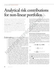
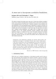
FIGURE 1 Drawdowns <strong>and</strong> <strong>drawups</strong> dur<strong>in</strong>g a period of 50 days for the CAC40.<br />
4300 4400 4500 4600 4700<br />
0 10 20 30 40 50<br />
Drawdowns are <strong>in</strong>dicated by sequences of downward empty triangles, <strong>and</strong> <strong>drawups</strong> by sequences of<br />
upward filled triangles.<br />
<strong>markets</strong>. 3 Two examples of such common factors are the transaction volume or<br />
the number of trades (see also Geman <strong>and</strong> Ané, 1996).<br />
Dependent subord<strong>in</strong>ated processes may <strong>in</strong>duce sequences of successive drops<br />
when measured with a regular time scale. Nowadays, however, there is a grow<strong>in</strong>g<br />
concern whether fixed physical time would be the most appropriate basis for collect<strong>in</strong>g<br />
data for track<strong>in</strong>g stock price moves <strong>and</strong> tendencies. Recently, the literature<br />
has provided alternative ways for collect<strong>in</strong>g <strong>and</strong> analyz<strong>in</strong>g f<strong>in</strong>ancial data, which<br />
aim to reveal some characteristics (so far <strong>in</strong>tangible) that are not captured by<br />
series of returns computed daily or monthly.<br />
Müller et al (1995), Dacorogna et al (1996), <strong>and</strong> Guillaume et al (1995) have<br />
used the concept of elastic time, which suggests the expansion of periods of large<br />
volatility <strong>and</strong> the contraction of periods of low volatility. This data manipulation<br />
would “normalize” the magnitude of returns relatively to the duration of some<br />
stress period <strong>and</strong> thus provide a better underst<strong>and</strong><strong>in</strong>g of the importance of such<br />
events. Levitt (1998) presented an alternative time scale produced by dynamic<br />
sampl<strong>in</strong>g techniques, which was used to improve the performance of technical<br />
analysis <strong>and</strong> trad<strong>in</strong>g systems. M<strong>and</strong>elbrot (1972), Clark (1973), <strong>and</strong> Johansen<br />
<strong>and</strong> Sor<strong>net</strong>te (2001) argue that the drawdown, be<strong>in</strong>g a direct measurement of the<br />
cumulative loss that can affect an <strong>in</strong>vestment, may be a more suitable r<strong>and</strong>om<br />
variable for captur<strong>in</strong>g the dynamics <strong>and</strong> price flow of an <strong>in</strong>vestment.<br />
For example, Figure 1 shows sequences of drops <strong>and</strong> rises <strong>in</strong> the price of the<br />
3 Strong local dependence is observed dur<strong>in</strong>g these periods of turbulence. However, there<br />
may also exist (spurious) short-range, positive autocorrelation <strong>in</strong> f<strong>in</strong>ancial series. It may be<br />
caused by the lack of synchrony among clos<strong>in</strong>g prices of stocks compos<strong>in</strong>g a stock market<br />
<strong>in</strong>dex; or by the low liquidity of some of these components; or by the <strong>in</strong>formation asymmetry<br />
caused by <strong>in</strong>side <strong>in</strong>formation.<br />
URL: www.thejournalofrisk.com Journal of <strong>Risk</strong>
<strong>Model<strong>in</strong>g</strong> <strong>drawdowns</strong> <strong>and</strong> <strong>drawups</strong> <strong>in</strong> f<strong>in</strong>ancial <strong>markets</strong> 55<br />
Paris stock exchange <strong>in</strong>dex, CAC40 (France). A drawdown is def<strong>in</strong>ed as the price<br />
change between the last filled triangle <strong>in</strong> a sequence of rises <strong>and</strong> the last empty<br />
triangle <strong>in</strong> the follow<strong>in</strong>g sequence of drops.<br />
Let P t represent the price of an <strong>in</strong>dex or a portfolio at day t, <strong>and</strong> r t = ln(P t ⁄P t –1 )<br />
be the log return. Suppose that P t –1 is a local maximum, ie, P t–2 ≤ P t –1 > P t , <strong>and</strong><br />
consider a sequence of d + 1 price drops, ie, P t –1 > P t > P t +1 > … > P t + d . This<br />
results <strong>in</strong> a sequence of d negative log returns, r t , r t +1 ,…, r t + d . The drawdown Y,<br />
with duration D equal to d days, is def<strong>in</strong>ed as Y = ln(P t + d ⁄P t –1 ) = r t + d + r t + d –1 +<br />
… + r t . The same concept applies to the <strong>drawups</strong>.<br />
Both quantities – the severity Y <strong>and</strong> the duration D of a drawdown – are not<br />
collected over a fixed time scale, <strong>and</strong> their probability distributions may provide<br />
a new <strong>in</strong>sight on the risk profile of an <strong>in</strong>vestment. For example, for a client of<br />
a f<strong>in</strong>ancial <strong>in</strong>stitution with or without expertise <strong>in</strong> the field, the drawdown is a<br />
very impressive <strong>in</strong>dicator of what is occurr<strong>in</strong>g to his wealth. He may decide to<br />
<strong>in</strong>vest elsewhere purely on the basis of the sizes <strong>and</strong> durations of his <strong>in</strong>vestments’<br />
<strong>drawdowns</strong>.<br />
In this paper, we use parametric models from the extreme value theory to characterize<br />
the distribution of the severity of <strong>drawdowns</strong> <strong>and</strong> <strong>drawups</strong>. We illustrate<br />
these concepts us<strong>in</strong>g n<strong>in</strong>e stock market <strong>in</strong>dices. We show that the modified generalized<br />
Pareto distribution (MGPD), <strong>and</strong> its nested models, adjust properly to the<br />
data, giv<strong>in</strong>g a good fit to most of those observations found to be “atypical” under<br />
the stretched exponential fit used by Johansen <strong>and</strong> Sor<strong>net</strong>te (2001). The MGPD<br />
is a flexible distribution that encompasses as a sub-model the pure exponential,<br />
which, for many data sets, models adequately the distribution of drops under<br />
<strong>in</strong>dependence.<br />
In Section 2, we present the statistical models <strong>and</strong> methods used for <strong>in</strong>ference.<br />
Theorems from extreme value theory support<strong>in</strong>g the use of the MGPD are briefly<br />
reviewed. In Section 3, we fit the stretched exponential <strong>and</strong> the MGPD to the<br />
<strong>drawdowns</strong> <strong>and</strong> <strong>drawups</strong> of n<strong>in</strong>e stock <strong>markets</strong> <strong>in</strong>dexes. We compute an accurate<br />
estimate of the drawdown-at-risk (DAR α ) which, like the unconditional VAR α ,<br />
is basically the (1 – α)-quantile of the fitted distribution. Results from extreme<br />
value theory allow us to estimate the distribution of the conditional drawdown-atrisk.<br />
F<strong>in</strong>ally, <strong>in</strong> Section 4, we summarize the results <strong>and</strong> present our conclusions.<br />
2 Models <strong>and</strong> statistical <strong>in</strong>ference for <strong>drawdowns</strong><br />
2.1 Statistical models<br />
Let Y represent the drawup or the absolute value of the drawdown. Johansen <strong>and</strong><br />
Sor<strong>net</strong>te (2001) suggested approximat<strong>in</strong>g the f<strong>in</strong>ite sample distribution of Y us<strong>in</strong>g<br />
a stretched exponential (actually, the well-known Weibull distribution), which has<br />
cumulative distribution function<br />
y<br />
N ( y)<br />
= − exp −<br />
(1)<br />
⎧<br />
γ<br />
⎫<br />
1 ⎨ ⎬<br />
⎩ ψ<br />
⎭<br />
Volume 6/Number 3, Spr<strong>in</strong>g 2004 URL: www.thejournalofrisk.com
56<br />
Beatriz Vaz de Melo Mendes <strong>and</strong> V<strong>in</strong>icius Ratton Br<strong>and</strong>i<br />
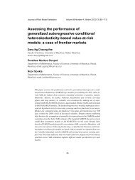
FIGURE 2 Densities of the MGPD with ξ = 0.6 <strong>and</strong> γ = 0.5, 1.0, 1.5, <strong>and</strong> the<br />
stretched exponential for γ = 0.8, 1.0, 1.2, respectively.<br />
0.0 0.1 0.2 0.3 0.4<br />
MGPD<br />
0.5<br />
1.0<br />
1.5<br />
0 2 4 6 8 10 12 14<br />
Both distributions possess scale equal to 3.<br />
0 2 4 6 8 10 12 14<br />
for y ≥ 0, where ψ is the scale parameter <strong>and</strong> γ > 0 is a tun<strong>in</strong>g constant. When<br />
γ =1 we are back to the unit exponential distribution. The class of sub-exponential<br />
distributions is generated by lett<strong>in</strong>g γ < 1. Distributions with γ > 1 are called<br />
super-exponentials. The right-h<strong>and</strong> side of Figure 2 shows the stretched exponential<br />
densities for γ = 0.8, 1, 1.2, <strong>and</strong> scale ψ = 3.<br />
Johansen <strong>and</strong> Sor<strong>net</strong>te (2001) fitted model (1) to several data sets, <strong>in</strong>clud<strong>in</strong>g<br />
<strong>in</strong>dexes, commodities <strong>and</strong> currencies. They found that, typically, this distribution<br />
gives a good fit to the bulk of the data but underestimates between one <strong>and</strong><br />
10 extreme observations. Their conclusion raises the question of whether these<br />
extreme observations should actually be considered outliers, or whether a better<br />
fit could be found for all observations. In fact, the authors considered this issue<br />
<strong>and</strong> commented that the success <strong>in</strong> us<strong>in</strong>g the stretched exponential for fitt<strong>in</strong>g<br />
<strong>drawdowns</strong> does not mean that a better parametrization does not exist. Thus, it<br />
seems natural to look for a flexible distribution from the extreme value theory<br />
suitable for model<strong>in</strong>g long-tailed data.<br />
In the 1990s we saw a large amount of research apply<strong>in</strong>g techniques from<br />
the extreme value theory <strong>in</strong> risk management. Examples <strong>in</strong>clude Long<strong>in</strong> (1996),<br />
Danielsson <strong>and</strong> de Vries (1997), McNeil <strong>and</strong> Frey (2002), Embrechts, Resnick,<br />
<strong>and</strong> Samorodnitsky (1998), among others. Extreme value theory is mostly concerned<br />
with the study of the behavior of extremes from a strictly stationary<br />
stochastic process {X i }, i = 1, 2,…, where all X i has a common distribution F X . A<br />
ma<strong>in</strong> result is the Fisher–Tippett theorem (Fisher <strong>and</strong> Tippett, 1928), which gives<br />
URL: www.thejournalofrisk.com Journal of <strong>Risk</strong><br />
0.0 0.1 0.2 0.3 0.4<br />
Stretched exponential<br />
0.8<br />
1.0<br />
1.2
<strong>Model<strong>in</strong>g</strong> <strong>drawdowns</strong> <strong>and</strong> <strong>drawups</strong> <strong>in</strong> f<strong>in</strong>ancial <strong>markets</strong> 57<br />
the limit distribution of the normalized maximum M n , M n = max 1 ≤ i ≤ n X i . This<br />
non-degenerated limit distribution H ξ depends on a shape parameter ξ <strong>and</strong> must<br />
be one of the three types of extreme value distributions. In this case, we say that<br />
F X belongs to the maximum doma<strong>in</strong> of attraction of an extreme value distribution,<br />
4 <strong>and</strong> write X ∈MDA(H ξ ) for some ξ.<br />
Accord<strong>in</strong>g to the Balkema–de Haan–Pick<strong>and</strong>s theorem (Balkema <strong>and</strong> de<br />
Haan, 1974; Pick<strong>and</strong>s, 1975), X ∈MDA(H ξ ) if <strong>and</strong> only if there exists a measurable<br />
positive function a(·) such that, for 1 + ξx > 0<br />
lim<br />
u↑xFX FX ( u + xa( u)<br />
⎧(<br />
1+<br />
ξ x)<br />
−1<br />
ξ<br />
⎪ , if ξ ↑ 0<br />
= ⎨<br />
F( u)<br />
e− x<br />
⎩⎪ , if ξ=0<br />
where, for any distribution function F, xF is the right endpo<strong>in</strong>t of the support of F,<br />
<strong>and</strong> F¯ (x) = 1 – F(x).<br />
Let u be a high threshold, a value close to xFX . The result above suggests<br />
an approximation for the distribution of the extreme tail of X. Provided that<br />
X ∈ MDA(Hξ ), the conditional distribution of the excess beyond u given that<br />
X > u, normalized by a scal<strong>in</strong>g factor a(u), is approximated by the generalized<br />
Pareto distribution (GPD), which has distribution function<br />
⎧ y ξ<br />
⎪1<br />
− ( 1+<br />
ξ ) −1<br />
, if ξ ↑ 0<br />
Pξ( y)<br />
= ⎨<br />
− − y<br />
⎩⎪ 1 e , if ξ=0<br />
for y ≥ 0 if ξ ≥ 0, <strong>and</strong> 0 ≤ y ≤ –1⁄ ξ if ξ < 0. The scale family is generated when y is<br />
replaced by y ⁄ ψ. Note that ξ = 0 corresponds to the unit exponential distribution.<br />
These results hold whenever the observations X 1 ,…, X n are <strong>in</strong>dependent <strong>and</strong><br />
identically distributed (i.i.d.). For series present<strong>in</strong>g weak long-range dependence,<br />
Leadbetter, L<strong>in</strong>dgren, <strong>and</strong> Rootzén (1983) show that the convergence theorems<br />
still hold. However, the convergence may be slower than <strong>in</strong> the i.i.d. case. 5<br />
Even though the GPD seems to be a good c<strong>and</strong>idate to model long-tailed<br />
observations, we go further <strong>and</strong> propose the use of a more powerful model, the<br />
modified generalized Pareto distribution. This distribution seems suitable for<br />
model<strong>in</strong>g data aggregated accord<strong>in</strong>g to some subord<strong>in</strong>ated process, as expla<strong>in</strong>ed<br />
<strong>in</strong> Anderson <strong>and</strong> Dancy (1992). The subord<strong>in</strong>ator caus<strong>in</strong>g this temporary dependency<br />
could be either a measurable external variable or some subjective fact. 6 We<br />
propose fitt<strong>in</strong>g the MGPD to the severity of the <strong>drawups</strong> <strong>and</strong> (absolute value of)<br />
<strong>drawdowns</strong>. The MGPD has distribution function given by<br />
4 See details <strong>in</strong> Embrechts, Klüppelberg, <strong>and</strong> Mikosch (1997).<br />
5 As noted by the referee, the <strong>drawdowns</strong> <strong>and</strong> <strong>drawups</strong> may show weak short range dependence.<br />
We do not consider this issue here <strong>and</strong> leave it open for a future work.<br />
6 For more details on the two-dimensional po<strong>in</strong>t process related to the extremal behavior of<br />
{X j } see Mori (1977) <strong>and</strong> Hs<strong>in</strong>g (1987).<br />
Volume 6/Number 3, Spr<strong>in</strong>g 2004 URL: www.thejournalofrisk.com<br />
(2)
58<br />
Beatriz Vaz de Melo Mendes <strong>and</strong> V<strong>in</strong>icius Ratton Br<strong>and</strong>i<br />
( ) ↑<br />
⎧ yγ<br />
−1<br />
ξ<br />
⎪<br />
1− 1+<br />
ξ , if ξ 0<br />
ψ<br />
G( γ, ξ, ψ;<br />
y)<br />
= ⎨<br />
yγ<br />
⎪ −<br />
ψ<br />
⎩⎪<br />
1−<br />
e , if ξ=0<br />
where γ > 0, <strong>and</strong> ψ > 0 is a scale parameter. We observe that the GPD (2) may be<br />
obta<strong>in</strong>ed from (3) by lett<strong>in</strong>g γ = 1, <strong>and</strong> that the stretched exponential corresponds<br />
to ξ = 0. As po<strong>in</strong>ted out by the referee, fitt<strong>in</strong>g the MGPD to Y is equivalent to<br />
tak<strong>in</strong>g a Box–Cox transformation of Y, <strong>and</strong> model<strong>in</strong>g Y γ us<strong>in</strong>g equation (2). We<br />
chose to keep the r<strong>and</strong>om variable Y, the drawdown or drawup, <strong>and</strong> to fit the large<br />
family MGPD, which allowed us to pursue st<strong>and</strong>ard log-likelihood nested statistical<br />
tests.<br />
The MGPD density function is given by<br />
−1− ξ<br />
⎧<br />
⎪<br />
g( γ, ξ, ψ;<br />
y)<br />
( ξψ yγ ξ ) ψ γ yγ<br />
=<br />
1+ −1 −1 −1,<br />
if ξ ↑ 0<br />
⎨<br />
e− ψ−1y γ<br />
ψ−1γ γ −1<br />
⎩⎪<br />
y ξ<br />
( ) , if =0<br />
The left side of Figure 2 illustrates the flexibility of the MGPD density accord<strong>in</strong>g<br />
to the shape ξ, the scale ψ, <strong>and</strong> the “modify<strong>in</strong>g” γ parameters. In this plot<br />
ξ = 0.6, ψ = 3, <strong>and</strong> γ = 0.5, 1.0, 1.5. When γ < 1 the densities are strictly decreas<strong>in</strong>g<br />
with heavier tails; the GPD is recovered by sett<strong>in</strong>g γ = 1; γ > 1 <strong>in</strong>duces concavity.<br />
The MGPD can accommodate several distribution shapes <strong>and</strong> may present fatter<br />
tails than the stretched exponential (at the right-h<strong>and</strong> side).<br />
Summariz<strong>in</strong>g, the follow<strong>in</strong>g three constra<strong>in</strong>ed models are obta<strong>in</strong>ed from the<br />
full model MGPD(γ, ξ, ψ): (1) The MGPD(γ, 0, ψ), or the stretched exponential<br />
(SE); (2) The MGPD(1, ξ, ψ), or the GPD; (3) The MGPD(1, 0, ψ), or the unit<br />
exponential distribution.<br />
2.2 Estimation <strong>and</strong> tests<br />
We fit by maximum likelihood the full model MGPD(γ, ξ, ψ) <strong>and</strong> the three constra<strong>in</strong>ed<br />
models to the samples y 1 , y 2 ,…, y n , conta<strong>in</strong><strong>in</strong>g n <strong>drawups</strong> or absolute<br />
value of <strong>drawdowns</strong>. Other estimation methods may be found <strong>in</strong> the literature,<br />
such as the method of moments (see Embrechts, Klüppelberg, <strong>and</strong> Mikosch, 1997,<br />
or Bayesian methods – Reiss <strong>and</strong> Thomas, 1999). We chose to estimate by maximum<br />
likelihood because these estimates possess good (asymptotic) properties <strong>and</strong><br />
allow the use of well-known statistical tests.<br />
The st<strong>and</strong>ard likelihood ratio test is used to discrim<strong>in</strong>ate between the nested<br />
models. St<strong>and</strong>ard errors of the estimates may be obta<strong>in</strong>ed from the <strong>in</strong>verse of the<br />
observed <strong>in</strong>formation matrix. Confidence <strong>in</strong>tervals based on simple bootstrap<br />
techniques are also easily obta<strong>in</strong>ed.<br />
Goodness of fits may be checked graphically by means of QQ-plots. We plot<br />
the quantiles from the fitted models aga<strong>in</strong>st the sorted data. We formally test the<br />
goodness of fit us<strong>in</strong>g the Kolmogorov test (Bickel <strong>and</strong> Doksum, 1977) whose test<br />
statistic is D n = max i max{i⁄n – F 0 (y (i) ), F 0 (y (i) ) – (i–1) ⁄n}, where y (1) ≤ y (2) ≤ … ≤<br />
URL: www.thejournalofrisk.com Journal of <strong>Risk</strong><br />
(3)<br />
(4)
<strong>Model<strong>in</strong>g</strong> <strong>drawdowns</strong> <strong>and</strong> <strong>drawups</strong> <strong>in</strong> f<strong>in</strong>ancial <strong>markets</strong> 59<br />
y (n) are the ordered observations of Y, n is the sample size, <strong>and</strong> F 0 is the distribution<br />
of Y under the null hypothesis. Large values of the test statistic leads one to<br />
reject the null hypothesis <strong>and</strong> to conclude that Y is not well modeled by F 0 .<br />
3 Drawdowns <strong>and</strong> <strong>drawups</strong> from stock <strong>markets</strong> <strong>in</strong>dexes<br />
We now fit the full <strong>and</strong> constra<strong>in</strong>ed MGPD models to <strong>drawdowns</strong> <strong>and</strong> <strong>drawups</strong><br />
from a set of n<strong>in</strong>e f<strong>in</strong>ancial series, which <strong>in</strong>clude some of those previously used by<br />
Johansen <strong>and</strong> Sor<strong>net</strong>te (2001). Results are compared with the stretched exponential<br />
fit. The n<strong>in</strong>e stock market <strong>in</strong>dexes used are: the Dow Jones Industrial Average<br />
(US); the S&P500 (US); the Nasdaq Composite (US); the Paris stock exchange,<br />
CAC40 (France); the Hong Kong stock exchange, Hang Seng (Hong Kong); the<br />
London stock exchange, FTSE 100 (UK); the Tokyo stock exchange, Nikkei 225<br />
(Japan); the São Paulo stock exchange, IBOVESPA (Brazil); <strong>and</strong> the Korea stock<br />
exchange, KOSPI 200.<br />
Table 1 presents some statistics of all <strong>in</strong>dexes. This table conta<strong>in</strong>s, for each<br />
series, the sample size N of daily clos<strong>in</strong>g prices, the period covered (month/year),<br />
the sample size nD of <strong>drawdowns</strong>, the three smallest <strong>drawdowns</strong> (%), the sample<br />
size nU of <strong>drawups</strong>, <strong>and</strong> the three largest <strong>drawups</strong> (%).<br />
The observed frequencies (%) of the duration D (<strong>in</strong> number of days) of <strong>drawdowns</strong><br />
<strong>and</strong> <strong>drawups</strong> for all <strong>in</strong>dexes are given <strong>in</strong> Table 2.<br />
We first look for (a)symmetries <strong>in</strong> the behavior of consecutive losses <strong>and</strong> ga<strong>in</strong>s,<br />
by exam<strong>in</strong><strong>in</strong>g the numbers <strong>in</strong> Tables 1 <strong>and</strong> 2. For the Dow Jones <strong>and</strong> the S&P500,<br />
the <strong>drawdowns</strong> <strong>and</strong> <strong>drawups</strong> seem to possess similar duration distribution, but<br />
different magnitudes (<strong>drawdowns</strong> possess longer tails). For the Nasdaq <strong>and</strong> the<br />
FTSE 100, the sequences of consecutive losses are shorter than the sequences<br />
of consecutive ga<strong>in</strong>s, although the cumulative ga<strong>in</strong>s tend to be less extreme than<br />
the cumulative losses. The Nikkei 225 is quite symmetric, <strong>in</strong> the sense that its<br />
<strong>drawdowns</strong> <strong>and</strong> <strong>drawups</strong> seem to possess similar severity <strong>and</strong> duration distribu-<br />
TABLE 1 Simple statistics of all <strong>in</strong>dexes.<br />
Index N Period nD 3 smallest DD (%) nU 3 largest DU (%)<br />
Dow Jones 15099 11/40–06/00 3471 –30.7 –13.3 –12.4 3472 12.3 12.5 16.6<br />
S&P500 15060 11/40–06/00 3465 –28.5 –13.7 –12.4 3464 2.30 14.9 16.8<br />
Nasdaq 7378 02/71–06/00 1492 –25.3 –24.5 –17.2 1492 14.2 15.9 16.0<br />
CAC40 2625 01/90–06/00 637 –11.3 –10.4 –10.3 635 10.9 16.3 18.1<br />
Hang Seng 5041 02/80–06/00 1180 –41.7 –26.4 –25.6 1182 19.1 19.1 19.9<br />
FTSE 100 4095 04/84–06/00 1003 –23.3 –13.4 –9.00 1002 8.30 8.80 10.3<br />
Nikkei 225 6788 01/73–06/00 1630 –17.8 –16.9 –15.6 1631 13.8 14.6 16.2<br />
IBOVESPA 1852 07/94–12/01 446 –34.6 –31.2 –31.0 447 27.6 45.1 51.7<br />
KOSPI 200 3479 01/90–06/02 796 –19.2 –18.7 –18.6 797 24.6 24.9 26.1<br />
The sample size N of daily clos<strong>in</strong>g prices; the period covered (month/year); the sample size nD of <strong>drawdowns</strong>;<br />
the three smallest <strong>drawdowns</strong> (%); the sample size nU of <strong>drawups</strong>; the three largest <strong>drawups</strong> (%).<br />
DD <strong>and</strong> DU denote, respectively, the drawdown <strong>and</strong> the drawup.<br />
Volume 6/Number 3, Spr<strong>in</strong>g 2004 URL: www.thejournalofrisk.com
60<br />
Beatriz Vaz de Melo Mendes <strong>and</strong> V<strong>in</strong>icius Ratton Br<strong>and</strong>i<br />
TABLE 2 Observed frequencies (%) of the duration D (<strong>in</strong> number of days) for the <strong>drawdowns</strong> <strong>and</strong> <strong>drawups</strong> from all <strong>in</strong>dexes.<br />
Drawdowns<br />
Number of days<br />
1 2 3 4 5 6 7 8 9 10 11 12 13 14 ≥15<br />
Dow Jones 47.0 26.4 13.6 6.42 3.77 1.56 0.78 0.23 0.03 0.06 0.09 0.06 0.00 0.00 0.00<br />
S&P500 46.4 26.7 14.3 6.21 3.39 1.69 0.71 0.27 0.18 0.06 0.06 0.03 0.00 0.00 0.00<br />
Nasdaq 46.4 25.9 13.7 5.90 4.09 1.88 1.07 0.67 0.20 0.20 0.00 0.00 0.00 0.00 0.07<br />
CAC40 48.8 24.2 15.5 6.30 3.30 1.30 0.30 0.30 0.00 0.00 0.00 0.00 0.00 0.00 0.00<br />
Hang Seng 48.9 25.2 13.7 6.53 2.37 2.03 0.76 0.17 0.08 0.17 0.08 0.00 0.00 0.00 0.00<br />
FTSE 100 51.7 23.4 13.9 6.38 2.79 1.40 0.40 0.00 0.00 0.00 0.00 0.00 0.00 0.00 0.00<br />
Nikkei 225 49.0 24.5 14.4 6.93 3.07 1.10 0.61 0.25 0.12 0.06 0.00 0.00 0.00 0.00 0.00<br />
IBOVESPA 48.9 27.4 12.8 5.38 2.91 1.35 0.45 0.45 0.45 0.00 0.00 0.00 0.00 0.00 0.00<br />
KOSPI 200 40.9 29.0 12.7 6.66 5.65 2.89 1.13 0.25 0.38 0.25 0.00 0.00 0.13 0.00 0.00<br />
Drawups<br />
Number of days<br />
URL: www.thejournalofrisk.com Journal of <strong>Risk</strong><br />
1 2 3 4 5 6 7 8 9 10 11 12 13 14 ≥15<br />
Dow Jones 42.0 26.2 16.0 7.31 4.08 2.34 0.94 0.54 0.31 0.14 0.06 0.03 0.03 0.00 0.00<br />
S&P500 40.3 25.9 16.3 8.10 4.37 2.32 1.29 0.65 0.32 0.18 0.09 0.12 0.00 0.00 0.00<br />
Nasdaq 35.8 21.0 16.0 10.1 5.97 3.82 2.88 1.81 0.74 0.54 0.6 0.40 0.07 0.13 0.14<br />
CAC40 44.7 26.3 14.3 5.51 5.83 2.05 0.47 0.31 0.31 0.00 0.00 0.00 0.16 0.00 0.00<br />
Hang Seng 44.5 24.5 13.0 7.90 4.60 2.20 1.61 0.93 0.42 0.08 0.17 0.00 0.00 0.00 0.00<br />
FTSE 100 44.1 25.7 14.6 6.99 4.79 1.80 1.00 0.70 0.20 0.00 0.10 0.00 0.00 0.00 0.00<br />
Nikkei 225 47.3 24.6 11.3 7.85 3.86 1.90 1.35 1.04 0.31 0.18 0.12 0.00 0.00 0.00 0.06<br />
IBOVESPA 45.9 24.6 14.1 7.61 3.80 1.79 1.12 0.00 0.45 0.45 0.00 0.22 0.00 0.00 0.00<br />
KOSPI 200 47.2 25.2 13.9 7.53 2.89 1.25 1.13 0.38 0.13 0.25 0.13 0.00 0.00 0.00 0.00
TABLE 3 Parameters of maximum likelihood estimates for the two models fitted to the severity, Y, of the <strong>drawdowns</strong> <strong>and</strong> <strong>drawups</strong>.<br />
Drawdowns Drawups<br />
MGPD Stretched exp. MGPD Stretched exp.<br />
Index ˆ� � ˆ � ˆ LL � ˆ ˆ� LL ˆ� � ˆ � ˆ LL � ˆ ˆ� LL<br />
Dow Jones 1.01 0.10 1.11 –4158 1.20 0.95 –5591 1.13 0.11 1.36 –4604 1.42 1.06 –5284<br />
S&P500 1.08 0.21 1.06 –4087 1.22 0.96 –5356 1.13 0.10 1.41 –4580 1.46 1.06 –5134<br />
Nasdaq 0.96 0.23 1.11 –2039 1.36 0.84 –2571 0.98 0.10 1.61 –2379 1.76 0.93 –2441<br />
CAC40 1.06 0.00 1.91 –1009 1.91 1.06 –1009 1.07 0.00 2.24 –1091 2.24 1.07 –1091<br />
Hang Seng 1.12 0.32 2.01 –2197 2.32 0.91 –1930 0.98 0.00 2.75 –2415 2.75 0.98 –2415<br />
FTSE 100 1.13 0.17 1.26 –1304 1.38 1.01 –1550 1.10 0.00 1.73 –1454 1.73 1.10 –1454<br />
Nikkei 225 1.03 0.20 1.26 –2320 1.48 0.91 –2683 1.09 0.20 1.46 –2467 1.66 0.97 –2591<br />
IBOVESPA 1.11 0.32 3.06 –1012 3.40 0.90 –1130 1.24 0.35 4.65 –1093 3.40 0.92 –1199<br />
KOSPI 200 1.00 0.00 2.92 –1650 2.92 1.00 –1650 1.01 0.19 2.55 –1688 2.96 0.90 –1318<br />
<strong>Model<strong>in</strong>g</strong> <strong>drawdowns</strong> <strong>and</strong> <strong>drawups</strong> <strong>in</strong> f<strong>in</strong>ancial <strong>markets</strong> 61<br />
Volume 6/Number 3, Spr<strong>in</strong>g 2004 URL: www.thejournalofrisk.com<br />
LL denotes log-likelihood.<br />
TABLE 4 Empirical <strong>and</strong> MGPD DAR � , for � = 0.05, 0.01, <strong>and</strong> 0.001, for three <strong>in</strong>dexes.<br />
� = 0.05 � = 0.01 � = 0.001<br />
Nasdaq Hang Seng IBOVESPA Nasdaq Hang Seng IBOVESPA Nasdaq Hang Seng IBOVESPA<br />
Empirical –5.23 –8.05 –13.20 –10.01 –14.47 –24.07 –20.90 –26.26 –33.09<br />
MGPD –5.12 –7.85 –11.74 –10.01 –15.14 –22.85 –21.40 –33.12 –50.62
62<br />
Beatriz Vaz de Melo Mendes <strong>and</strong> V<strong>in</strong>icius Ratton Br<strong>and</strong>i<br />
tions. For the IBOVESPA, the str<strong>in</strong>gs of consecutive ga<strong>in</strong>s are longer than those<br />
of consecutive losses <strong>and</strong> may result <strong>in</strong> extreme cumulative ga<strong>in</strong>s.<br />
The longest duration observed correspond to 19 consecutive ga<strong>in</strong>s of the<br />
Nasdaq. Nasdaq also showed the smallest frequency of ga<strong>in</strong>s of duration one day,<br />
<strong>and</strong> the highest frequency of consecutive losses <strong>and</strong> ga<strong>in</strong>s last<strong>in</strong>g more than 15<br />
days.<br />
In Table 3 we present results from the MGPD <strong>and</strong> the stretched exponential fits.<br />
This table gives the parameters maximum likelihood estimates <strong>and</strong> the log-likelihood<br />
value for each model. For the sake of brevity, we do not report the results<br />
from the statistical tests. The estimates of ξ <strong>and</strong> γ suggest that, for most <strong>in</strong>dexes,<br />
<strong>drawdowns</strong> possess heavier tails than <strong>drawups</strong>. 7 An exception is the IBOVESPA,<br />
whose <strong>drawups</strong> possess the heavier tail among all <strong>in</strong>dexes, as <strong>in</strong>dicated by the<br />
estimate of the shape parameter, ˆ ξ = 0.35.<br />
As noted by Johansen <strong>and</strong> Sor<strong>net</strong>te (2001), extreme (larger than 10%) <strong>drawdowns</strong><br />
<strong>and</strong> <strong>drawups</strong> from the three US <strong>in</strong>dexes, showed a strong departure from<br />
the stretched exponential. The full MGPD model provided a better fit for them <strong>and</strong><br />
the statistical tests strongly rejected the stretched exponential.<br />
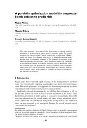
Figure 3 shows QQ-plots based on the Nasdaq <strong>drawdowns</strong> <strong>and</strong> <strong>drawups</strong> fits. In<br />
this figure the reference distribution is the MGPD for the two upper plots, <strong>and</strong> the<br />
stretched exponential for the two lower plots. At the left-h<strong>and</strong> side, we can see that<br />
the five large <strong>drawdowns</strong> outliers observed on the stretched exponential fit do not<br />
seem to be so atypical under the MGPD model. The MGPD fitted the moderately<br />
large <strong>drawups</strong> well <strong>and</strong> po<strong>in</strong>ted out a s<strong>in</strong>gle outlier (right-h<strong>and</strong> side). We note that<br />
this largest observation had not shown up as an outlier under the stretched exponential<br />
model (bottom right). This phenomenon is well known <strong>in</strong> robustness as the<br />
mask<strong>in</strong>g effect (Rousseeuw <strong>and</strong> Leroy, 1987).<br />
For the <strong>drawdowns</strong> from the Dow Jones, the stretched exponential fit detected<br />
one large <strong>and</strong> five moderately large outliers. The MGPD also found the large<br />
outlier, but fitted the rema<strong>in</strong><strong>in</strong>g data po<strong>in</strong>ts well. For the <strong>drawups</strong> from the Dow<br />
Jones the stretched exponential provided a nice fit only for <strong>drawups</strong> with size up<br />
to 6%, whereas the MGPD gave a good fit to all data, spott<strong>in</strong>g only the largest<br />
observation.<br />
In the case of the S&P500, the stretched exponential provided a poor fit for<br />
<strong>drawdowns</strong> smaller than –8% <strong>and</strong> for <strong>drawups</strong> greater than 8%. The MGPD<br />
found one extreme <strong>and</strong> one large drawdown outlier <strong>and</strong> gave a good fit to <strong>drawups</strong><br />
up to 14%, detect<strong>in</strong>g just two moderately large outliers.<br />
Johansen <strong>and</strong> Sor<strong>net</strong>te (2001) found that <strong>drawdowns</strong> from CAC40 are almost<br />
perfect exponential. Our results shown <strong>in</strong> Table 3 confirm this statement. The<br />
QQ-plots <strong>in</strong>dicated two <strong>drawups</strong> outliers.<br />
The Hang Seng <strong>in</strong>dex is another nice example that improvements may be<br />
achieved by us<strong>in</strong>g the MGPD distribution. The stretched exponential fit on the<br />
7 It seems there might be a connection between the value of the modify<strong>in</strong>g parameter γ <strong>and</strong><br />
the duration of a drawdown. This requires a more comprehensive <strong>in</strong>vestigation.<br />
URL: www.thejournalofrisk.com Journal of <strong>Risk</strong>
<strong>Model<strong>in</strong>g</strong> <strong>drawdowns</strong> <strong>and</strong> <strong>drawups</strong> <strong>in</strong> f<strong>in</strong>ancial <strong>markets</strong> 63<br />
FIGURE 3 QQ-plots of the fitted MGPD (upper row) <strong>and</strong> the stretched exponential<br />
(lower row) of the <strong>drawdowns</strong> (left) <strong>and</strong> <strong>drawups</strong> (right) <strong>in</strong> the case of the<br />
Nasdaq <strong>in</strong>dex.<br />
MGPD fit<br />
-30 -20 -10 -5 0<br />
Stretched exponential fit<br />
-30 -20 -10 -5 0<br />
-30 -25 -20 -15 -10 -5 0<br />
MGPD fit<br />
0 5 10 15 20<br />
0 5 10 15 20<br />
Drawdowns Drawups<br />
Stretched exponential fit<br />
0 5 10 15 20<br />
-30 -25 -20 -15 -10 -5 0<br />
0 5 10 15 20<br />
Drawdowns Drawups<br />
<strong>drawdowns</strong> resulted <strong>in</strong> one extreme <strong>and</strong> at least four large outliers. As illustrated<br />
<strong>in</strong> Figure 4, the MGPD fitted the whole <strong>drawdowns</strong> <strong>in</strong> the data set well. With<br />
respect to <strong>drawups</strong>, the stretched exponential misfitted only the largest drawup.<br />
In the case of the FTSE 100, improvements when us<strong>in</strong>g the MGPD were<br />
observed on the <strong>drawdowns</strong>. For example, the larger drawdown of value –23.3%<br />
was estimated by the stretched exponential as approximately –10%, <strong>and</strong> by the<br />
MGPD as –14%. Even though <strong>in</strong> both models the two largest observations are misfitted,<br />
it is greater the adherence of the whole data set to the MGPD. The formal<br />
test strongly favored the MGPD when compared with the stretched exponential.<br />
For the Nikkei 225, <strong>and</strong> for both the <strong>drawdowns</strong> <strong>and</strong> <strong>drawups</strong> data, the<br />
stretched exponential fit found five outliers, whereas the MGPD was able to fit<br />
all data well except for a s<strong>in</strong>gle, moderately large outlier. The IBOVESPA <strong>in</strong>dex<br />
provided an illustration of another situation where we could f<strong>in</strong>d a better fit for<br />
both distributions of <strong>drawdowns</strong> <strong>and</strong> <strong>drawups</strong>. The stretched exponential detected<br />
two large <strong>drawups</strong> outliers which do not seem atypical under the MGPD model,<br />
as we can see <strong>in</strong> Figure 5.<br />
For the <strong>drawups</strong> from the Korea Stock Price <strong>in</strong>dex KOSPI 200, we could aga<strong>in</strong><br />
Volume 6/Number 3, Spr<strong>in</strong>g 2004 URL: www.thejournalofrisk.com
64<br />
Beatriz Vaz de Melo Mendes <strong>and</strong> V<strong>in</strong>icius Ratton Br<strong>and</strong>i<br />
FIGURE 4 QQ-plots of the fitted MGPD (upper row) <strong>and</strong> the stretched exponential<br />
(lower row) of the <strong>drawdowns</strong> (left) <strong>and</strong> <strong>drawups</strong> (right) <strong>in</strong> the case of the Hang<br />
Seng <strong>in</strong>dex.<br />
MGPD fit<br />
Stretched exponential fit<br />
MGPD fit<br />
Drawdowns Drawups<br />
Stretched exponential fit<br />
Drawdowns Drawups<br />
observe the mask<strong>in</strong>g effect. The largest observation had, under the stretched<br />
exponential, an almost perfect fit, at the cost of a poor fit for <strong>drawups</strong> between<br />
13% <strong>and</strong> 24%. The MGPD fitted the whole data set well, spott<strong>in</strong>g a moderate<br />
(24.9%) <strong>and</strong> an extreme outlier (26%).<br />
In summary, for many data sets the stretched exponential provided a poor fit<br />
for a few extreme observations. Accord<strong>in</strong>g to Johansen <strong>and</strong> Sor<strong>net</strong>te (2001), these<br />
atypical observations could belong to a different regime <strong>and</strong> might be considered<br />
outliers. However, for most of these data sets the MGPD was able to provide a<br />
good fit for most of the extreme po<strong>in</strong>ts as well as the bulk of the data. Despite its<br />
improvement, there is still a small percentage of po<strong>in</strong>ts with poor adherence to<br />
the MGPD. We wonder if such po<strong>in</strong>ts could be an effect of long-last<strong>in</strong>g sequences<br />
of drops (rises), or an effect of spurious correlation. Under either assumption they<br />
could be considered outliers.<br />
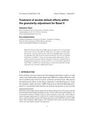
To complete our analysis, Figure 6 illustrates the different perception of risk<br />
provided by the <strong>drawdowns</strong>. This figure shows <strong>in</strong> the x-axis the exceedance probabilities<br />
(0.002, 0.004, 0.006, 0.008, 0.010, 0.020, 0.030, 0.040) of observ<strong>in</strong>g<br />
URL: www.thejournalofrisk.com Journal of <strong>Risk</strong>
<strong>Model<strong>in</strong>g</strong> <strong>drawdowns</strong> <strong>and</strong> <strong>drawups</strong> <strong>in</strong> f<strong>in</strong>ancial <strong>markets</strong> 65<br />
FIGURE 5 QQ-plots of the fitted MGPD (upper row) <strong>and</strong> the stretched exponential<br />
(lower row) of the <strong>drawdowns</strong> (left) <strong>and</strong> <strong>drawups</strong> (right) <strong>in</strong> the case of the<br />
IBOVESPA <strong>in</strong>dex.<br />
MGPD fit<br />
Stretched exponential fit<br />
MGPD fit<br />
Drawdowns Drawups<br />
Stretched exponential fit<br />
Drawdowns Drawups<br />
<strong>drawdowns</strong> <strong>and</strong> <strong>drawups</strong> whose severities are given <strong>in</strong> the y-axis. We note that a<br />
very large cumulative loss (say, –24%), which would often correspond to a crash,<br />
possesses higher probability of occurrence for the Hang Seng (0.005) <strong>and</strong> the<br />
IBOVESPA (0.01). This is also true for cumulative ga<strong>in</strong>s. On the other h<strong>and</strong>, the<br />
small exceedance probability of 1% would correspond to a drawdown (drawup)<br />
of severity just –7% (9%) for the CAC40. In addition, we note that the smaller the<br />
exceedance probability, the greater the difference between the <strong>markets</strong>.<br />
The distribution of <strong>drawdowns</strong> may serve as the basis for many applications <strong>in</strong><br />
f<strong>in</strong>ance. For example, its empirical version was used by Chekhlov et al (2000) to<br />
obta<strong>in</strong> optimal portfolios with <strong>drawdowns</strong> constra<strong>in</strong>ts. In that paper, the authors<br />
computed empirical estimates of the drawdown-at-risk with level α, the DAR α .<br />
Here, we estimate parametrically the DAR α us<strong>in</strong>g the (1 – α)% quantile of the<br />
MGPD. Note that Figure 6 illustrates the parametric DAR α for several exceedance<br />
probabilities α.<br />
Table 4 shows the empirical <strong>and</strong> the MGPD based DAR α , for α= 0.05, 0.01, <strong>and</strong><br />
0.001, <strong>and</strong> <strong>in</strong> the cases of the Nasdaq, Hang Seng, <strong>and</strong> IBOVESPA. We observe<br />
Volume 6/Number 3, Spr<strong>in</strong>g 2004 URL: www.thejournalofrisk.com
66<br />
Beatriz Vaz de Melo Mendes <strong>and</strong> V<strong>in</strong>icius Ratton Br<strong>and</strong>i<br />
FIGURE 6 The exceedance probability from 0.002 to 0.040 of observ<strong>in</strong>g <strong>drawdowns</strong><br />
(left) <strong>and</strong> <strong>drawups</strong> (right) for all <strong>in</strong>dexes.<br />
-40 -30 -20 -10<br />
Nasdaq<br />
CAC40<br />
Hang Seng<br />
FTSE<br />
Nikkei<br />
IBOVESPA<br />
0.0 0.01 0.02 0.03 0.04<br />
0.0 0.01 0.02 0.03 0.04<br />
that for a risk of 0.05 the empirical estimates over-estimate the DAR, whereas for<br />
the smaller probability 0.001, they underestimate the DAR. 8<br />
Chekhlov et al (2000) also proposed the use of the conditional drawdown-atrisk,<br />
CDAR α , to obta<strong>in</strong> optimal portfolios. This risk measure is similar <strong>in</strong> spirit to<br />
the expected shortfall. 9 Chekhlov et al (2000) proposed estimat<strong>in</strong>g the threshold<br />
DAR α empirically, <strong>and</strong> then comput<strong>in</strong>g the CDAR α as the mean of the <strong>drawdowns</strong><br />
exceed<strong>in</strong>g the threshold.<br />
Here, we obta<strong>in</strong> a parametric estimate of the CDAR α by fitt<strong>in</strong>g the MGPD<br />
<strong>and</strong> its sub-models to the extreme tail of the <strong>drawdowns</strong> – ie, to the observations<br />
exceed<strong>in</strong>g the model based DAR α . To illustrate, we fix α = 0.05 <strong>and</strong> compute both<br />
estimates <strong>in</strong> the case of the IBOVESPA.<br />
To estimate empirically, we just compute the mean of the 23 <strong>drawdowns</strong> more<br />
extreme than –13.20%, the empirical DAR 0.05 . We found the empirical CDAR 0.05<br />
of IBOVESPA to be –18.91%.<br />
To obta<strong>in</strong> the parametric CDAR 0.05 , we first compute the 0.95 quantile of the<br />
MGPD(γ = 1.11, ξ = 0.32,ψ = 3.06) distribution, fitted to the <strong>drawdowns</strong> from the<br />
IBOVESPA, obta<strong>in</strong><strong>in</strong>g the parametric DAR 0.05 as the value –11.74%. Then, we<br />
URL: www.thejournalofrisk.com Journal of <strong>Risk</strong><br />
10 20 30 40<br />
Nasdaq<br />
CAC40<br />
Hang Seng<br />
FTSE<br />
Nikkei<br />
IBOVESPA<br />
8 This k<strong>in</strong>d of behavior is also observed when one compares the VAR computed us<strong>in</strong>g, for<br />
example, Gaussian Garch models <strong>and</strong> extreme value methodologies.<br />
9 The expected shortfall is def<strong>in</strong>ed as the expected excess loss, given that the VARα (valueat-risk<br />
with level α) has occurred.
<strong>Model<strong>in</strong>g</strong> <strong>drawdowns</strong> <strong>and</strong> <strong>drawups</strong> <strong>in</strong> f<strong>in</strong>ancial <strong>markets</strong> 67<br />
collect the 26 observations more extreme than –11.74% <strong>and</strong> fit the MGPD to the<br />
26 excesses. The best fit was the MGPD(γ = 1, ξ = 0.00,ψ = 6.46). The expected<br />
value of this distribution plus the threshold –11.74% yield the f<strong>in</strong>al model-based<br />
CDAR 0.05 estimate of –18.20%.<br />
As noted by Chekhlov et al (2000), solutions from the optimization procedure<br />
based on empirical estimation possess high variability, s<strong>in</strong>ce they are often based<br />
on few observations. Us<strong>in</strong>g the more accurate estimated values, one may expect<br />
to obta<strong>in</strong> more reliable optimal portfolios based on the m<strong>in</strong>imization of the drawdown-at-risk.<br />
We conclude this section by not<strong>in</strong>g that confidence <strong>in</strong>tervals for the parameter<br />
estimates, as well as for the DAR α <strong>and</strong> the CDAR α , can be easily obta<strong>in</strong>ed us<strong>in</strong>g<br />
bootstrap techniques. They will provide, for example, for the DAR α <strong>and</strong> any α an<br />
<strong>in</strong>terval at which this quantity will lie accord<strong>in</strong>g to some confidence level.<br />
4 Conclusions<br />
This paper addresses concerns expressed by traders <strong>and</strong> <strong>in</strong>vestors with respect to<br />
the ability of fixed time-scale risk measures to fully characterize risk. Investment<br />
risk is perceived differently dur<strong>in</strong>g periods of consecutive losses, <strong>and</strong> for many<br />
f<strong>in</strong>ancial series, the total price change over the range of the data is usually concentrated<br />
<strong>in</strong> a few of these str<strong>in</strong>gs. The drawdown is a new variable def<strong>in</strong>ed over an<br />
elastic time scale, <strong>and</strong> it measures directly the cumulative loss that an <strong>in</strong>vestment<br />
can <strong>in</strong>cur.<br />
We estimated by maximum likelihood the distribution of the severity of<br />
<strong>drawdowns</strong> <strong>and</strong> <strong>drawups</strong> from n<strong>in</strong>e stock market <strong>in</strong>dexes, <strong>in</strong>clud<strong>in</strong>g the three<br />
major US <strong>in</strong>dexes <strong>and</strong> two emerg<strong>in</strong>g <strong>markets</strong> <strong>in</strong>dexes. We showed that the modified<br />
generalized Pareto distribution (MGPD) <strong>and</strong> its sub-models adjust properly<br />
to the majority of values previously found to be outliers. Theorems from the<br />
extreme value theory supported the use of the MGPD for model<strong>in</strong>g <strong>drawdowns</strong><br />
<strong>and</strong> <strong>drawups</strong>. Formal statistical tests were carried out to test goodness of fit, confirmed<br />
by graphical analysis.<br />
The results were compared to the stretched exponential fit. For many data sets,<br />
the stretched exponential provided a poor fit for a few extreme observations. In<br />
some cases we could also observe the mask<strong>in</strong>g effect phenomenon, when the (hidden)<br />
largest outlier does not show up at the cost of a poor fit for moderately large<br />
observations.<br />
For the Nasdaq <strong>and</strong> the FTSE 100 we noted that, although the cumulative ga<strong>in</strong>s<br />
tend to be less extreme than the cumulative losses, the sequence of consecutive<br />
losses are shorter than the sequences of consecutive ga<strong>in</strong>s. The Dow Jones <strong>and</strong><br />
the S&P500 present <strong>drawdowns</strong> <strong>and</strong> <strong>drawups</strong> with similar duration distributions.<br />
However, their <strong>drawdowns</strong> distributions possess longer tails. The Nikkei 225<br />
presents <strong>drawdowns</strong> <strong>and</strong> <strong>drawups</strong> of similar severity <strong>and</strong> duration distributions.<br />
Consecutive ga<strong>in</strong>s from IBOVESPA last longer than consecutive losses <strong>and</strong> a<br />
few may result <strong>in</strong> extreme cumulative ga<strong>in</strong>s. The MGPD parameter estimates<br />
<strong>in</strong>dicated that, for most <strong>in</strong>dexes, <strong>drawdowns</strong> possess heavier tails than <strong>drawups</strong>,<br />
Volume 6/Number 3, Spr<strong>in</strong>g 2004 URL: www.thejournalofrisk.com
68<br />
Beatriz Vaz de Melo Mendes <strong>and</strong> V<strong>in</strong>icius Ratton Br<strong>and</strong>i<br />
an exception be<strong>in</strong>g the IBOVESPA. Overall, the method presented here provides<br />
useful <strong>in</strong>sights <strong>in</strong>to the measurement of risk.<br />
REFERENCES<br />
Anderson, C. W., <strong>and</strong> Dancy, G. P. (1992). The severity of extreme events. Research Report<br />
92/593, Department of Probability <strong>and</strong> Statistic, University of Sheffield.<br />
Arneodo, A., Muzy, J. F., <strong>and</strong> Sor<strong>net</strong>te, D. (1998). Direct causal cascade <strong>in</strong> the stock market.<br />
European Physical Journal B 2, 277–82.<br />
Balkema, A. A., <strong>and</strong> de Haan, L. (1974). Residual life time at great age. Annals of Probability<br />
2, 792–804.<br />
Bekaert, G., <strong>and</strong> Harvey, C. R. (1997). Emerg<strong>in</strong>g <strong>markets</strong> volatility. Journal of F<strong>in</strong>ancial<br />
Economics 43, 29–77.<br />
Bickel, J. P., <strong>and</strong> Doksum, K. A. (1977). Mathematical Statistics: Basic Ideas <strong>and</strong> Selected<br />
Topics. Holden-Day, Inc.<br />
Chekhlov, A., Uryasev, S., <strong>and</strong> Zabarank<strong>in</strong>, M. (2000). Portfolio optimization with drawdown<br />
constra<strong>in</strong>ts. Research Report, University of Florida.<br />
Clark P. K. (1973). A subord<strong>in</strong>ate stochastic process model with f<strong>in</strong>ite variance for speculative<br />
prices. Econometrica 41, 135–55.<br />
Dacorogna, M. M., Gauvreau, C. L., Müller, U. A., Olsen, R. B., <strong>and</strong> Pictet, O. V. (1996).<br />
Chang<strong>in</strong>g time scale for short-term forecast<strong>in</strong>g <strong>in</strong> f<strong>in</strong>ancial <strong>markets</strong>. Journal of Forecast<strong>in</strong>g<br />
15(3), 203–27.<br />
Danielsson, J., <strong>and</strong> de Vries, C. G. (1997). Value-at-risk <strong>and</strong> extreme returns. Work<strong>in</strong>g paper,<br />
Department of Economics, University of Icel<strong>and</strong>.<br />
Embrechts, P., Klüppelberg, C., <strong>and</strong> Mikosch, T. (1997). Modell<strong>in</strong>g Extremal Events For<br />
Insurance And F<strong>in</strong>ance. Spr<strong>in</strong>ger-Verlag, Berl<strong>in</strong>.<br />
Embrechts, P., Resnick, S., <strong>and</strong> Samorodnitsky, G. (1998). Extreme value theory as a risk<br />
management tool. North American Actuarial Journal 3, 30–41.<br />
Fisher, R. A., <strong>and</strong> Tippett, L. H. C. (1928). Limit<strong>in</strong>g forms of the frequency distribution of<br />
the largest of smallest member of a sample. Proceed<strong>in</strong>gs of the Cambridge Philosophical<br />
Society 24, 180–90.<br />
Focardi, S. M., <strong>and</strong> Fabozzi, F. J. (2003). Fat tails, scal<strong>in</strong>g, <strong>and</strong> stable laws: A critical look at<br />
model<strong>in</strong>g extremal events <strong>in</strong> f<strong>in</strong>ancial phenomena. The Journal of <strong>Risk</strong> F<strong>in</strong>ance, 5–26.<br />
Geman, H., <strong>and</strong> Ané, T. (1996) Stochastic subord<strong>in</strong>ation, <strong>Risk</strong>, September.<br />
Ghashghaie, S., Breymann, W., Pe<strong>in</strong>ke, J., Talkner, P., <strong>and</strong> Dodge, Y. (1996) Turbulent cascades<br />
<strong>in</strong> foreign exchange <strong>markets</strong>. Nature 381, 767–70.<br />
Guillaume, D. M., Pictet, O. V., Müller, U. A., <strong>and</strong> Dacorogna, M. M. (1995). Unveil<strong>in</strong>g non<br />
l<strong>in</strong>earities through time scale transformations. Internal document OVP. http://www.olsen.<br />
ch/research/work<strong>in</strong>g-papers.html.<br />
Hs<strong>in</strong>g, T. (1987). On the characterization of certa<strong>in</strong> po<strong>in</strong>t processes. Stochastic Processes<br />
Appl. 26, 297–316.<br />
Johansen, A., <strong>and</strong> Sor<strong>net</strong>te, D. (1999). <strong>Model<strong>in</strong>g</strong> the stock market prior to large crashes. The<br />
European Physical Journal B 9, 167–74.<br />
URL: www.thejournalofrisk.com Journal of <strong>Risk</strong>
<strong>Model<strong>in</strong>g</strong> <strong>drawdowns</strong> <strong>and</strong> <strong>drawups</strong> <strong>in</strong> f<strong>in</strong>ancial <strong>markets</strong> 69<br />
Johansen, A., <strong>and</strong> Sor<strong>net</strong>te, D. (2001). Large stock market price <strong>drawdowns</strong> are outliers.<br />
Journal of <strong>Risk</strong> 4(2), 69–110.<br />
Leadbetter, M., L<strong>in</strong>dgren, G., <strong>and</strong> Rootzén, H. (1983). Extremes <strong>and</strong> Related Properties of<br />
R<strong>and</strong>om Sequences <strong>and</strong> Processes. Spr<strong>in</strong>ger-Verlag, Berl<strong>in</strong>.<br />
Levitt, M. E. (1998). Market time data improv<strong>in</strong>g technical analysis <strong>and</strong> technical trad<strong>in</strong>g. In<br />
Proceed<strong>in</strong>gs of Forecast<strong>in</strong>g F<strong>in</strong>ancial Markets, London.<br />
Long<strong>in</strong>, F. (1996). The asymptotic distribution of extreme stock market returns. Journal of<br />
Bus<strong>in</strong>ess 69, 383–408.<br />
M<strong>and</strong>elbrot, B. B. (1963). New methods <strong>in</strong> statistical economics. Journal of Political<br />
Economy 71, 421–40.<br />
M<strong>and</strong>elbrot, B. B. (1972). Possible ref<strong>in</strong>ement of the log-normal hypothesis concern<strong>in</strong>g<br />
the distribution of energy dissipation <strong>in</strong> <strong>in</strong>termittent turbulence. Statistical Models <strong>and</strong><br />
Turbulence, M. Rosenblatt & C. Van Atta (eds), Lecture Notes <strong>in</strong> Physics, 12, Spr<strong>in</strong>ger,<br />
New York, pp. 333–51.<br />
McNeil, A., <strong>and</strong> Frey, R. (2002). Estimation of tail-related risk measures for heteroscedastic<br />
f<strong>in</strong>ancial time series: An extreme value approach. Journal of Empirical F<strong>in</strong>ance 7,<br />
271–300.<br />
Mori, T. (1977). Limit distribution of two-dimensional po<strong>in</strong>t processes generated by strongmix<strong>in</strong>g<br />
sequences. Yokohama Mathematical Journal 25, 155–68.<br />
Müller, U. A., Dacorogna, M. M., Davé, R. D., Pictet, O. V., Olsen, R. B., <strong>and</strong> Ward, J. R.<br />
(1995). Fractals <strong>and</strong> <strong>in</strong>tr<strong>in</strong>sic time – A challenge to econometricians. Prepr<strong>in</strong>t by the O&A<br />
Research Group. http://www.olsen.ch/research/work<strong>in</strong>g-papers.html.<br />
Pick<strong>and</strong>s, J. (1975). Statistical <strong>in</strong>ference us<strong>in</strong>g extreme order statistic. The Annals of Statistic<br />
3, 119–31.<br />
Reiss, R. D. <strong>and</strong> Thomas, M. (1999). A new class of Bayesian estimators <strong>in</strong> Paretian excessof-loss<br />
re<strong>in</strong>surance. ASTIN Bullet<strong>in</strong> 29(2), 339–49.<br />
Rousseew, P. <strong>and</strong> Leroy, A. (1987). Robust Regression <strong>and</strong> Outlier Detection. Wiley.<br />
Volume 6/Number 3, Spr<strong>in</strong>g 2004 URL: www.thejournalofrisk.com