endof-

More documents

Recommendations

Info

Chapter 10 The DFT and the FFT AlgorithmIts value on the unit circle of the z -plane, is∞∑Fz ( ) = f [ n]z – nn = 0(10.1)( ) = f [ n]e njFe jωT∞∑n = 0(10.2)This represents an infinite summation; it must be truncated before it can be computed. Let thistruncated version be represented by– ωTN–1∑Xm [ ] = xn [ ]en = 0– j2π mn -------N(10.3)where N represents the number of points that are equally spaced in the interval 0 to 2π on theunit circle of the z -plane, andω =⎛ 2π------- ⎞ m⎝ NT⎠for m= 012… , , , , N – 1. We refer to relation (10.3) as the N – point DFT of X [ m].The Inverse DFT is defined asxn [ ]=N – 11--- X [ m]eN ∑m = 0j2π mn -------N(10.4)for n = 0, 1, 2 , …,N – 1.In general, the discrete frequency transformX [ m]is complex, and thus we can express it asX [ m] = Re{ X [ m]} + Im{ X [ m]}(10.5)for m=012… , , , , N – 1.Sincewe can express (10.3) ase– j2π mn -------N=cos2πmn-------------- – jsin--------------2πmnN N(10.6)N – 1∑– j2π mn -------NX [ m] = x[ n]e=n = 0N – 12πmn2πmn∑x[ n]cos -------------- – j x[ n]sin--------------N ∑ Nn = 0N – 1n = 0(10.7)10−2Signals and Systems with MATLAB ® Computing and Simulink ® Modeling, Fourth EditionCopyright © Orchard Publications
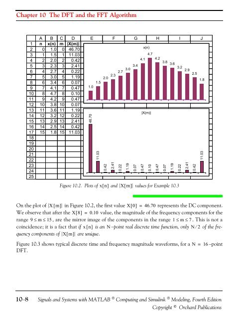
Chapter 10 The DFT and the FFT Algorithm12345678910111213141516171819202122232425A B C D E F G H I Jn x(n) m |X(m)|0 1.0 0 46.70x(n)1 1.5 1 11.034.72 2.0 2 0.424.1 4.23 2.3 3 2.413.44 2.7 4 0.225 3.0 5 1.192.0 2.3 2.7 3.0 3.8 3.63.2 2.92.56 3.4 6 0.07 1.57 4.1 7 0.471.08 4.7 8 0.109 4.2 9 0.4710 3.8 10 0.0711 3.6 11 1.1912 3.2 12 0.22|X(m)|13 2.9 13 2.4114 2.5 14 0.4215 1.8 15 11.0346.7011.030.422.410.221.190.070.470.100.470.071.190.222.410.421.811.03Figure 10.2. Plots of xn [ ] and Xm [ ] values for Example 10.3On the plot of X[ m] in Figure 10.2, the first value X0 [ ] = 46.70 represents the DC component.We observe that after the X8 [ ] = 0.10 value, the magnitude of the frequency components for therange 9≤ m≤ 15, are the mirror image of the components in the range 1 ≤ m≤7. This is not acoincidence; it is a fact that if x[ n] is an N−point real discrete time function, only N ⁄ 2 of the frequencycomponents of Xm [ ] are unique.Figure 10.3 shows typical discrete time and frequency magnitude waveforms, for aDFT.N = 16−point10−8Signals and Systems with MATLAB ® Computing and Simulink ® Modeling, Fourth EditionCopyright © Orchard Publications
Page 7: 4.2 Complex Impedance Z(s).........
Page 10 and 11: 8.6.4 The Transform of ft () = Acos
Page 12 and 13: 11.2.1 RC Low−Pass Filter .......
Page 14 and 15: MATLAB ComputingPages D−3, D−4,
Page 16 and 17: The Unit Step FunctionThus, the pul
Page 18 and 19: Chapter 1 Elementary Signals6. To d
Page 20 and 21: Chapter 2 The Laplace Transformatio
Page 22 and 23: Chapter 2 The Laplace Transformatio
Page 24 and 25: Chapter 3 The Inverse Laplace Trans
Page 26 and 27: Chapter 4Circuit Analysis with Lapl
Page 28 and 29: Solutions to End−of−Chapter Exe
Page 30 and 31: Chapter 5 State Variables and State
Page 32 and 33: A: [−1 −1; 3/4 0]B: [1 0]’C:
Page 38 and 39: Chapter 7 Fourier Seriesthat is, th
Page 40 and 41: Chapter 8 The Fourier Transform8.2
Page 42 and 43: Chapter 8 The Fourier TransformExam
Page 44 and 45: Chapter 9 Discrete−Time Systems a
Page 46 and 47: num=[0 1 0 0];% The coefficients of
Page 50 and 51: The Fast Fourier Transform (FFT)The
Page 52 and 53: Basic Analog Filters11.2.3 RLC Band
Page 54 and 55: Chapter 11 Analog and Digital Filte
Page 56 and 57: Digital Filters1Four signals separa
Page 58 and 59: Chapter 11 Analog and Digital Filte
Page 60: Appendix E Window Functionsh[n]A(f)
Page 63 and 64: Appendix E Window FunctionsMH 1 ( z
Page 65 and 66: IndexSymbols Cauchy’s residue the
Page 67 and 68: Fourier transform - properties of f
Page 69 and 70: S for discrete-time systems 9-45 St

endof-

You also want an ePaper? Increase the reach of your titles

Delete template?

Save as template?