Numerical Analysis

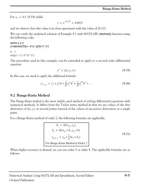
Forx 5 = 0.5(9.18) yieldsand we observe that this value is in close agreement with the value of (9.17).Runge-Kutta MethodWe can verify the analytical solution of Example 9.1 with MATLAB’s dsolve(s) function usingthe following code:syms x y zz=dsolve('Dy=−x*y','y(0)=1','x')z =exp(-1/2*x^2)y = e – 0.125 = 0.8825The procedure used in this example, can be extended to apply to a second order differentialequationy′′ = f( x, y,y ′)In this case, we need to apply the additional formula1y ′ i + 1y′ i y′′hi----y ′′′h 2 1 ( 4) 3= + +2! i + ----y3! i h +…(9.19)(9.20)9.2 Runge-Kutta MethodThe Runge-Kutta method is the most widely used method of solving differential equations withnumerical methods. It differs from the Taylor series method in that we use values of the firstderivative of f( x,y)at several points instead of the values of successive derivatives at a singlepoint.For a Runge-Kutta method of order 2, the following formulas are applicable.k 1 = hf( x n , y n )k 2 = hf( x n + h,y n + h)1y n + 1= y n + -- ( k2 1 + k 2 )For Runge-Kutta Method of Order 2(9.21)When higher accuracy is desired, we can use order 3 or order 4. The applicable formulas are asfollows:Numerical Analysis Using MATLAB and Spreadsheets, Second Edition 9-5Orchard Publications