Numerical Analysis

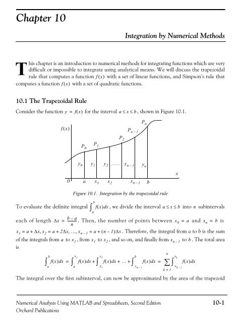
Chapter 10Integration by Numerical MethodsThis chapter is an introduction to numerical methods for integrating functions which are verydifficult or impossible to integrate using analytical means. We will discuss the trapezoidalrule that computes a function f ( x)with a set of linear functions, and Simpson’s rule thatcomputes a function f ( x)with a set of quadratic functions.10.1 The Trapezoidal RuleConsider the function y = f( x)for the interval a≤x≤b, shown in Figure 10.1.f ( x)P nP n – 1P 2PP 1 00y 0 y 1 y 2........... y n – 1 y nax 1 x 2x n – 1Figure 10.1. Integration by the trapezoidal rulebxbTo evaluate the definite integral∫fx , we divide the interval a ≤x ≤ b into n subintervalsaeach of length ∆xb–a= ----------- . Then, the number of points between xn0 = a and x n = b isx 1 = a + ∆x, x 2 = a+2∆x, …,x n – 1 = a+ ( n – 1)∆x. Therefore, the integral from a to b is the sumof the integrals from a to x 1 , from x 1 to x 2 , and so on, and finally from x n – 1 to b . The total areais∫abfx ( ) dx=∫fx ( ) dx+∫fx ( ) dx+ … +∫fx ( ) dx=∑ ∫fx ( ) dxax 1x 2x 1The integral over the first subinterval, can now be approximated by the area of the trapezoidbx n – 1nk = 1x kx k – 1Numerical Analysis Using MATLAB and Spreadsheets, Second Edition 10-1Orchard Publications